Day 9 Applied Linear Mixed Models I

June 15th, 2026

9.1 Announcements

• Homeworks review
  • “An RCBD is an experimental design used to reduce variability among experimental units”
• Initiating a hybrid approach in the next few weeks

9.2 Applied Linear Mixed Models

Today and Thursday, we’ll focus on the models behind most models for analyzing designed experiments.

9.2.1 Review: random variables

Data are typically considered a random variable (e.g., \(y\sim N(\mu, \sigma^2)\). Random variables are usually described with their properties like the expected value and variance. The expected value and variance are the first and second central moments of a distribution, respectively. Regardless of the distribution of a random variable \(y\), we could calculate its expected value \(E(y)\) and variance \(Var(y)\). The expected value measures the average outcome of \(y\). The variance measures the dispersion of \(y\), i.e. how far the possible outcomes are spread out from their average.

9.2.1.1 Demo: normally distributed random variable

9.2.1.2 Review: variance-covariance

The variance of a random variable can be conceived as the level of dispersion in a variable. The covariance between two random variables means how the two random variables behave relative to each other. Essentially, it quantifies the relationship between their joint variability. For example, the covariance between two variables \(y_1\) and \(y_2\) will make
Note that the variance of a random variable is the covariance of a random variable with itself. Consider two variables \(y_1\) and \(y_2\) each with a variance of 1 and a covariance of 0.6. Using the notation we’ve been using in class, that can be written as

\[\mathbf{y} \sim N (\boldsymbol{\mu}, \mathbf{V}),\]

where \(\mathbf{y}\) is the vector containing the variables \(y_1\) and \(y_2\), \(\mathbf{y} \equiv [y_1, y_2]'\), \(\boldsymbol{\mu}\) is the mean vector, \(\boldsymbol{\mu} \equiv [0,0]'\), and \(\mathbf{V}\) is the variance-covariance matrix. We can say that \(\mathbf{V} = \begin{bmatrix} 1 & 0.6 \\ 0.6 & 1\end{bmatrix}\).

set.seed(43)
# some covariance
mgcv::rmvn(1, c(0,0), matrix(c(1, .6, .6, 1), nrow=2, ncol=2))

## [1] -0.03751376 -1.28219179

mgcv::rmvn(1, c(0,0), matrix(c(1, .6, .6, 1), nrow=2, ncol=2))

## [1] -0.48596752  0.08056847

mgcv::rmvn(1, c(0,0), matrix(c(1, .6, .6, 1), nrow=2, ncol=2))

## [1] -0.9040981 -0.7644051

mgcv::rmvn(1, c(0,0), matrix(c(1, .6, .6, 1), nrow=2, ncol=2))

## [1] 0.3864344 0.1835374

# no covariance
mgcv::rmvn(1, c(0,0), matrix(c(1, 0, 0, 1), nrow=2, ncol=2))

## [1] -0.6861798 -1.9061368

mgcv::rmvn(1, c(0,0), matrix(c(1, 0, 0, 1), nrow=2, ncol=2))

## [1]  1.8037598 -0.9668729

mgcv::rmvn(1, c(0,0), matrix(c(1, 0, 0, 1), nrow=2, ncol=2))

## [1] -0.3531183  1.1069375

mgcv::rmvn(1, c(0,0), matrix(c(1, 0, 0, 1), nrow=2, ncol=2))

## [1] 0.5663244 2.0643087

9.3 Review: Designs

When we model data generated by designed experiments, we typically put the information from the treatment as affecting the mean (\(\mu\)), while the elements from the design (topographical, design, or the logistics of the experiment) indicate which observations are truly independent and which ones are not.

• Completely randomized designs: independent EUs
• Randomized complete block designs: groups of similar EUs

9.4 Split-plot designs

• Remember the definition of experimental unit? The smallest unit to which a treatment is independently applied.
• Sometimes we find that there are different sizes of experimental units.
• In such cases, it is important to identify the different experimental units and the randomization scheme. We may be in front of a multilevel design.

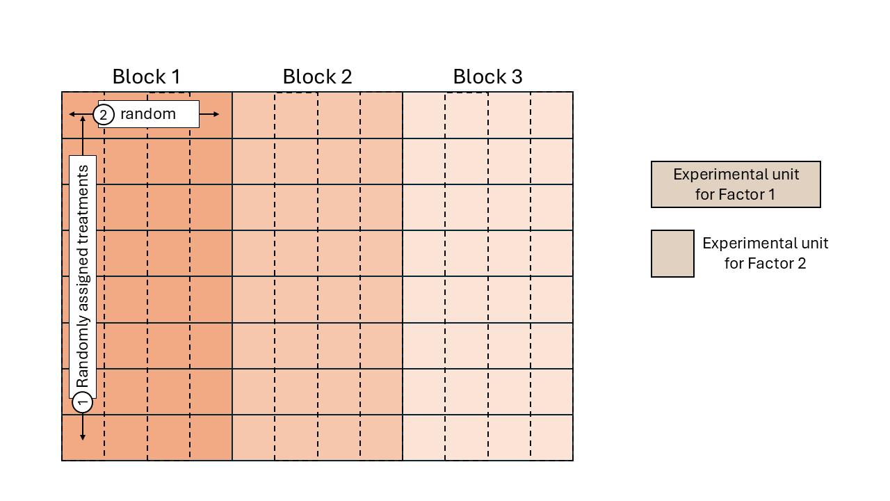
Figure 9.1: Schematic description of a field experiment with a split-plot design

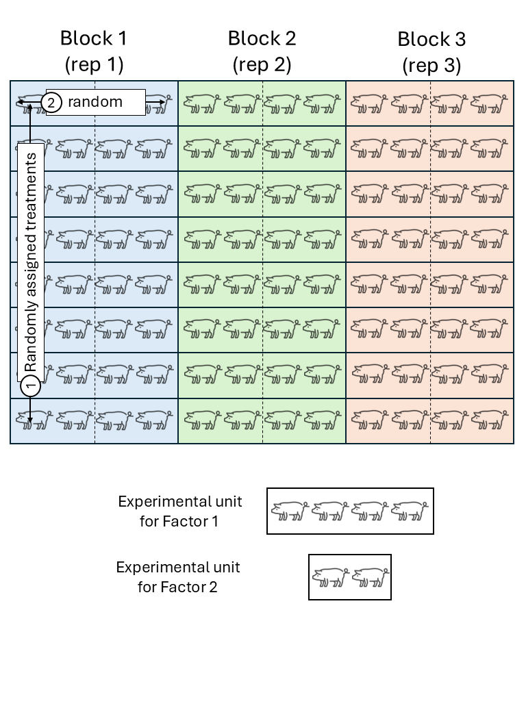
Figure 9.2: Schematic description of a swine experiment with a split-plot design

• Sometimes, these differences in the sizes of EUs are not that easy to notice.
  
• More details in Analysis of Messy Data - Ch5.