Day 10 Hierarchical (Multilevel) Designs
June 16th, 2025
10.1 Announcements
- Homework #2 is posted and due in a week.
- Office hours today are 11.20am-12pm.
- ONLINE class tomorrow (Wednesday 06-17)
10.2 Review: Hierarchical Designs
- Remember the definition of experimental unit? The smallest unit to which a treatment is independently applied.
- Sometimes we find that there are different sizes of experimental units.
- In such cases, it is important to identify the different experimental units and the randomization scheme. We may be in front of a multilevel design.
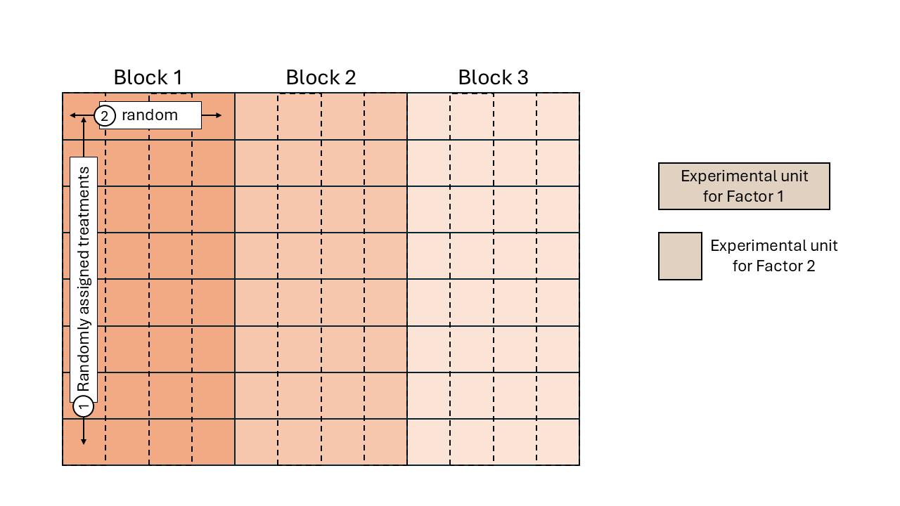
Figure 10.1: Schematic description of a field experiment with a split-plot design
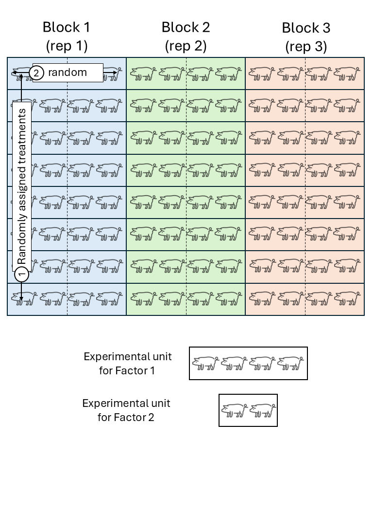
Figure 10.2: Schematic description of a swine experiment with a split-plot design
- Sometimes, these differences in the sizes of EUs are not that easy to notice.
- More details in Analysis of Messy Data - Ch5.
10.2.1 An applied example:
- Designed experiment of barley with fungicide treatments.
- Fungicide has some logistic restrictions that make it harder to apply the treatment in a small area only.
- Let’s take a look at the maps:
library(tidyverse)
library(agridat)
library(ggpubr)

data("durban.splitplot")
df <- durban.splitplot

theme_set(theme_minimal())

p_blocks <-
  df |>
  ggplot(aes(bed, row))+
  geom_tile(aes(fill = block))+
  geom_tile(color = "black", fill=NA)+
  coord_fixed()

p_wholeplot <-
  df |>
  ggplot(aes(bed, row))+
  geom_tile(aes(fill = fung))+
  geom_tile(color = "black", fill=NA)+
  coord_fixed()

p_splitplot <-
df |>
  ggplot(aes(bed, row))+
  geom_tile(aes(fill = gen), show.legend= F)+
  geom_tile(color = "black", fill=NA)+
  coord_fixed()

ggarrange(p_blocks, p_wholeplot, p_splitplot, ncol = 1, nrow = 3)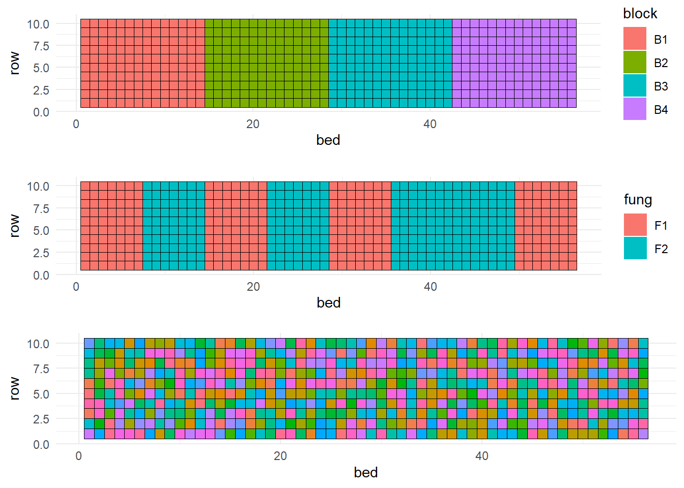
Rows and beds (aka columns) probably looked somewhat like this:

Discuss:
- Experimental units
- Observational units
- Treatment structure
- Design structure
- Could we have had the same treatment structure with a different design?
10.3 Building the ANOVA skeleton using design (aka topographical) and treatment elements
|
|
|
10.4 Blocks: fixed of random?
- The assumptions behind \(b_j\) vary:
- Fundamentals of mixed models
- Assumption behind blocks as fixed effects: there is a ‘true’ block effect out there.
- Assumption behind blocks as random effects:
- Confidence intervals of the means differ depending on the model:
- Blocks as fixed: \(\hat\mu \pm t \cdot \sqrt{\frac{\sigma_{\varepsilon}^2 }{b}}\)
- Blocks as random: \(\hat\mu \pm t \cdot \sqrt{\frac{\sigma_{\varepsilon}^2 + \sigma^2_{b}}{b}}\)
- Confidence intervals of the means differences don’t differ depending on the model:
- Blocks as fixed/as random: \(\hat\mu \pm t \cdot \sqrt{\frac{2 \sigma_{\varepsilon}^2 }{b}}\)
Some reading material:
- “Should blocks be fixed or random?” (Dixon, 2016)