Day 14 Review: hierarchical multilevel models – cont.
June 22nd, 2026
14.1 Announcements
Homework #2 due tomorrow
From the online poll:
- “I would like to have a better understanding of why df matters” – this week and next!
- “A split plot always need to have randomization?” – let’s go to day 2 (golden rules of designed experiments)
- “I would like to learn more about adaptive designs and/or bayesian experimental design (extra).” – STAT 870
14.2 Hierarchical designs
A study was designed to determine the effect on the incidence of root rot, of variety of wheat, kinds of dust for seed treatment, method of application of the dust, and efficacy of soil inoculation with the root-rot organism. We have a data frame with 160 observations on the following 8 variables that describe a designed experiment:
rowrow: equivalent to “longitude” in the field coordinatescolcolumn: equivalent to “latitude” in the field coordinatesyieldyield: response variableinocinoculate: indicator whether soil was inoculated with root rot or not
gengenotype treatmentdustdust treatmentdrydry or wet dust applicationblockblock: the field was divided in 4 equally-sized subsections that showed approximately similar characteristics.
Note that:
- The field has 4 areas of similar experimental units (blocks).
- Within each block, the genotype treatments were applied.
- Within each block-genotype, the dry-dust treatments were applied.
- Within each block-genotype-dry-dust, the inoculation treatments were applied.
14.3 Review
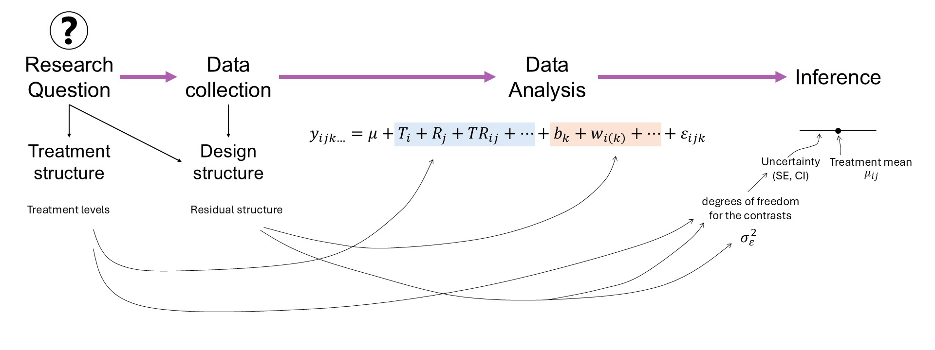
Figure 14.1: Mind map
14.3.1 Treatment structure
- What treatment factor(s) and/or combinations of treatment factors we’ve got.
- Typically defines the fixed effects in a model.
14.3.2 Design structure
- How we apply said treatment factors in practice (what are the experimental units?).
- Typically defines the random effects in a model.
Hierarchical designs
- Typically, different treatment factors have different EUs.
- Therefore, randomization ocurrs in nested structures.
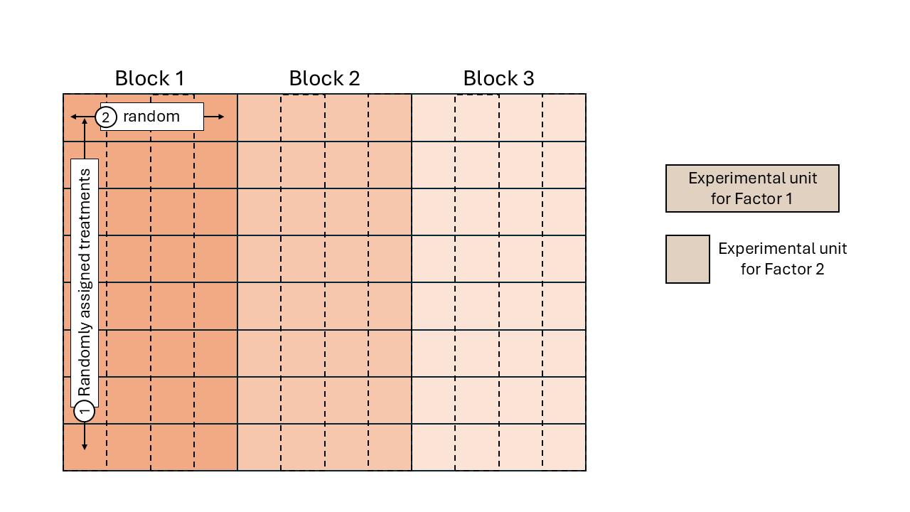
Figure 14.2: Schematic description of a field experiment with a split-plot design
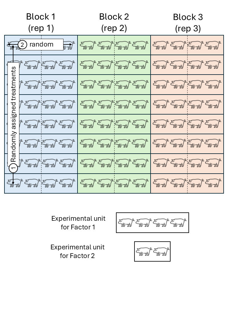
Figure 14.3: Schematic description of a swine experiment with a split-plot design
- The most common statistical model assumes:
- Constant variance,
- Normality,
- Independence – this changes with hierarchical designs! That’s why we use mixed models.
14.4 Exercises
Data structure
- Draw a figure of the structure in the data. Do not consider the treatments yet.
Designed experiment
2a. Draw a figure of the different randomization steps. 2b. Indicate the experimental units for the different treatment factors. 2c. How many observations do you have for each treatment factor? 2d. What are the treatment structure and the design structure?
Recall from day 2:
.](../figures/fisher_diagram.jpg)
Figure 14.4: Fisher’s diagram ‘The Principles of Field Experimentation’. Figure 1 in Preece (1990).
Stat model
3a. Write the statistical model that describes the data generating process. 3b. Fit the model in (3) to the data using R.
library(lme4)

m <- lmer(yield ~ inoc*gen*dry*dust + (1|block/gen/dry:dust), data = df)

performance::check_model(m, check = c("normality", "homogeneity"))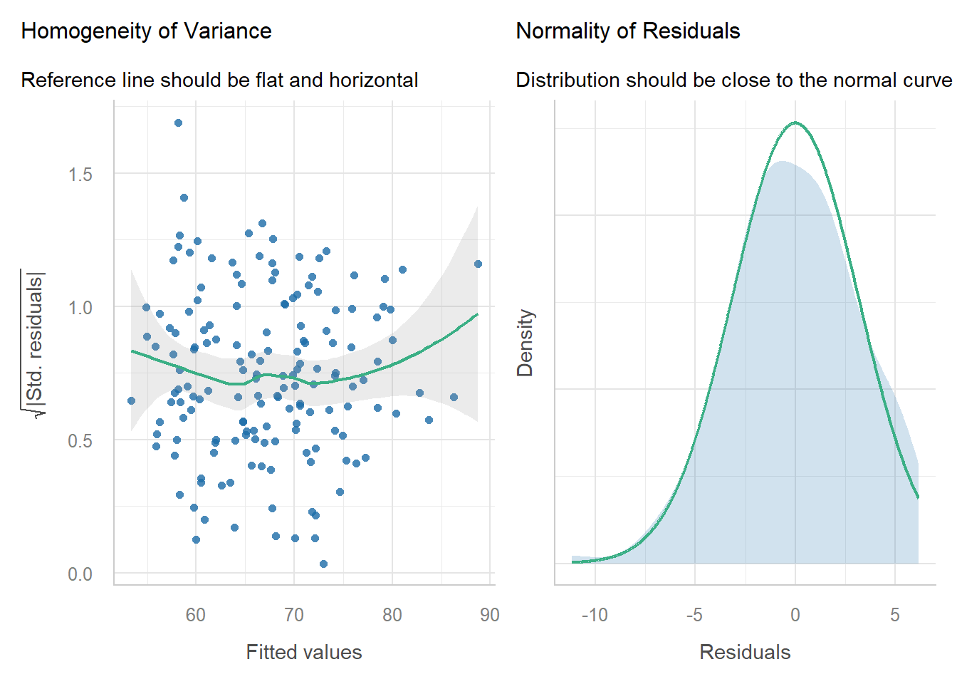
## Linear mixed model fit by REML ['lmerMod']
## Formula: yield ~ inoc * gen * dry * dust + (1 | block/gen/dry:dust)
##    Data: df
##
## REML criterion at convergence: 863.2
##
## Scaled residuals:
##      Min       1Q   Median       3Q      Max
## -2.84839 -0.53343 -0.00891  0.49012  1.57229
##
## Random effects:
##  Groups             Name        Variance Std.Dev.
##  dust:dry:gen:block (Intercept)  2.113   1.454
##  gen:block          (Intercept)  9.813   3.133
##  block              (Intercept)  2.849   1.688
##  Residual                       15.390   3.923
## Number of obs: 160, groups:  dust:dry:gen:block, 80; gen:block, 8; block, 4
##
## Fixed effects:
##                       Estimate Std. Error t value
## (Intercept)           67.11875    1.43578  46.747
## inoc1                  2.45625    0.31014   7.920
## gen1                  -4.76875    1.16154  -4.106
## dry1                   0.85625    0.35014   2.445
## dust1                  1.72500    0.70028   2.463
## dust2                 -2.02500    0.70028  -2.892
## dust3                  4.03750    0.70028   5.766
## dust4                 -2.36875    0.70028  -3.383
## inoc1:gen1             0.04375    0.31014   0.141
## inoc1:dry1            -0.65625    0.31014  -2.116
## gen1:dry1             -0.75625    0.35014  -2.160
## inoc1:dust1            0.70000    0.62027   1.129
## inoc1:dust2           -0.73750    0.62027  -1.189
## inoc1:dust3            2.70000    0.62027   4.353
## inoc1:dust4           -1.33125    0.62027  -2.146
## gen1:dust1             0.36250    0.70028   0.518
## gen1:dust2             0.30000    0.70028   0.428
## gen1:dust3            -1.88750    0.70028  -2.695
## gen1:dust4             0.45625    0.70028   0.652
## dry1:dust1            -0.07500    0.70028  -0.107
## dry1:dust2            -0.70000    0.70028  -1.000
## dry1:dust3             0.42500    0.70028   0.607
## dry1:dust4             0.76875    0.70028   1.098
## inoc1:gen1:dry1        0.15625    0.31014   0.504
## inoc1:gen1:dust1       0.86250    0.62027   1.391
## inoc1:gen1:dust2      -0.13750    0.62027  -0.222
## inoc1:gen1:dust3       0.42500    0.62027   0.685
## inoc1:gen1:dust4      -1.60625    0.62027  -2.590
## inoc1:dry1:dust1      -0.62500    0.62027  -1.008
## inoc1:dry1:dust2       0.06250    0.62027   0.101
## inoc1:dry1:dust3       0.56250    0.62027   0.907
## inoc1:dry1:dust4      -0.21875    0.62027  -0.353
## gen1:dry1:dust1        0.03750    0.70028   0.054
## gen1:dry1:dust2        0.22500    0.70028   0.321
## gen1:dry1:dust3        1.60000    0.70028   2.285
## gen1:dry1:dust4       -1.30625    0.70028  -1.865
## inoc1:gen1:dry1:dust1 -0.18750    0.62027  -0.302
## inoc1:gen1:dry1:dust2  0.06250    0.62027   0.101
## inoc1:gen1:dry1:dust3 -0.31250    0.62027  -0.504
## inoc1:gen1:dry1:dust4  0.15625    0.62027   0.252
varcomp <- VarCorr(m)
sigma2 <- sigma(m)^2
sigma2_b <- varcomp$block[1]
sigma2_wp <- varcomp$`gen:block`[1]
sigma2_sp <- varcomp$`dust:dry:gen:block`[1]
wp_n <- n_distinct(df$gen)
sp_n <- n_distinct(df$dry)*n_distinct(df$dust)
ssp_n <- n_distinct(df$inoc)
block_n <- n_distinct(df$block)
## se diff (whole plot factor)
sqrt(2*(sigma2 + ssp_n*sigma2_sp + ssp_n*sp_n*sigma2_wp)/(block_n*ssp_n*sp_n))## [1] 2.323079## contrast estimate SE df t.ratio p.value
## c(1, -1) -9.54 2.32 3 -4.106 0.0262
##
## Results are averaged over the levels of: inoc, dry, dust
## Degrees-of-freedom method: kenward-roger## [1] 1.56587## contrast estimate SE df t.ratio p.value
## c(1, -1, 0, 0, 0, 0, 0, 0, 0, 0) 1.56 1.57 54 0.998 0.3228
##
## Results are averaged over the levels of: inoc, gen
## Degrees-of-freedom method: kenward-roger## [1] 0.6202733## contrast estimate SE df t.ratio p.value
## c(1, -1) 4.91 0.62 60 7.920 <0.0001
##
## Results are averaged over the levels of: gen, dry, dust
## Degrees-of-freedom method: kenward-rogerBonus
- How would you name this experiment design?