Day 13 Statistical inference and experiment designs
JUne 23rd, 2026
13.2 Why do we care about standard errors and degrees of freedom?
13.2.1 The hypothesis test explanation
Typically (for a two-tailed test):
- Obtain t test statistic \(t^\star = \frac{\hat\theta}{se(\hat\theta)}\).
- Obtain \(t_c = t_{df, \ \alpha/2}\).
- Obtain \(P(t^\star>t_c)\).
- If \(P(t^\star>t_c) > \alpha\), reject \(H_0\).
13.2.2 The signal & noise explanation
- Each point estimate should be associated to some measure of uncertainty
- How little uncertainty do you need to be convinced?
- What is a 100% confidence interval (CI)? Why is it less useful than a 95% CI?
- A 95% CI tells us the range of values where we would not reject the null (Murtaugh, 2013).
13.2.3 Applied case I – CRD
A group of scientists ran an experiment to answer whether swine diets can affect the Serum haptoglobin concentration. The treatment structure was a \(6 \times 2\) factorial with Diet (6 levels) and Moment (2 levels) as the treamtment factors. The design structure was a CRD with 16 repetitions.
The scientists measured Serum haptoglobin (mg/dL) as the response variable and wish to maintain this metric as high as possible.
url <- "https://raw.githubusercontent.com/stat720/summer2026/refs/heads/main/data/blood_study_pigs.csv"
df <- read.csv(url) |>
  mutate(Trt = as.factor(Trt), Day = as.factor(Day))
Because this is a CRD, the model is
\[y_{ijk} = \mu_0 + T_i + D_j +(T\times D)_{ij} + \varepsilon_{ijk}, \\ \varepsilon_{ijk} \sim N(0, \sigma^2).\]
m <- lm(Serum_haptoglobin_mg.dL ~ Trt*Day, data = df)

performance::check_model(m,  check = c("normality", "homogeneity"))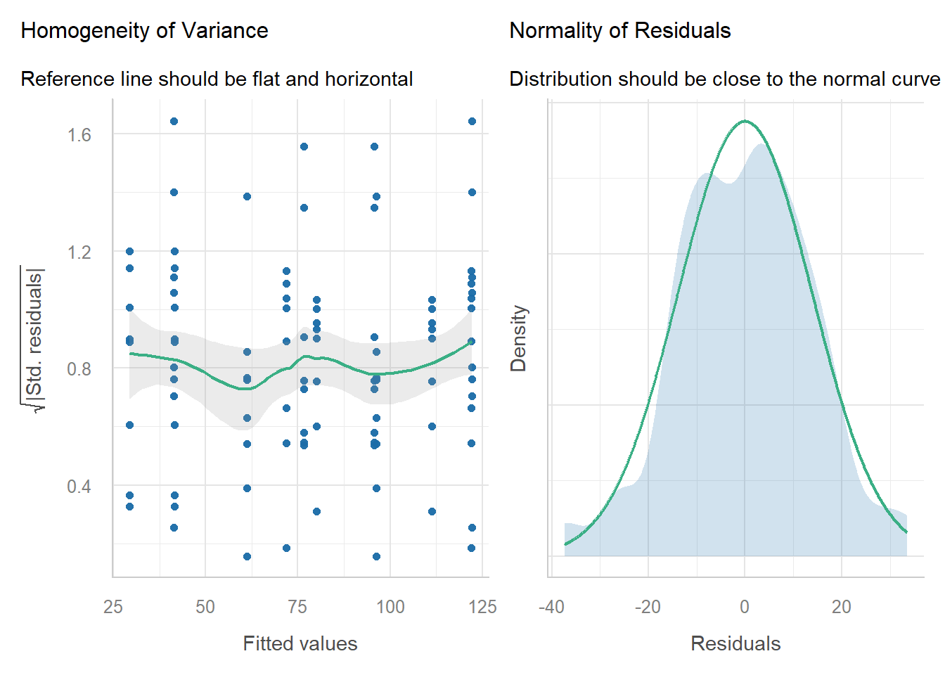
## Anova Table (Type II tests)
##
## Response: Serum_haptoglobin_mg.dL
##           Sum Sq  Df F value    Pr(>F)
## Trt        81720   5  80.049 < 2.2e-16 ***
## Day        69495   1 340.369 < 2.2e-16 ***
## Trt:Day    24352   5  23.854 < 2.2e-16 ***
## Residuals  36751 180
## ---
## Signif. codes:  0 '***' 0.001 '**' 0.01 '*' 0.05 '.' 0.1 ' ' 1
13.2.4 Biological significance (and others) matter as much as statistical significance
## NOTE: Results may be misleading due to involvement in interactions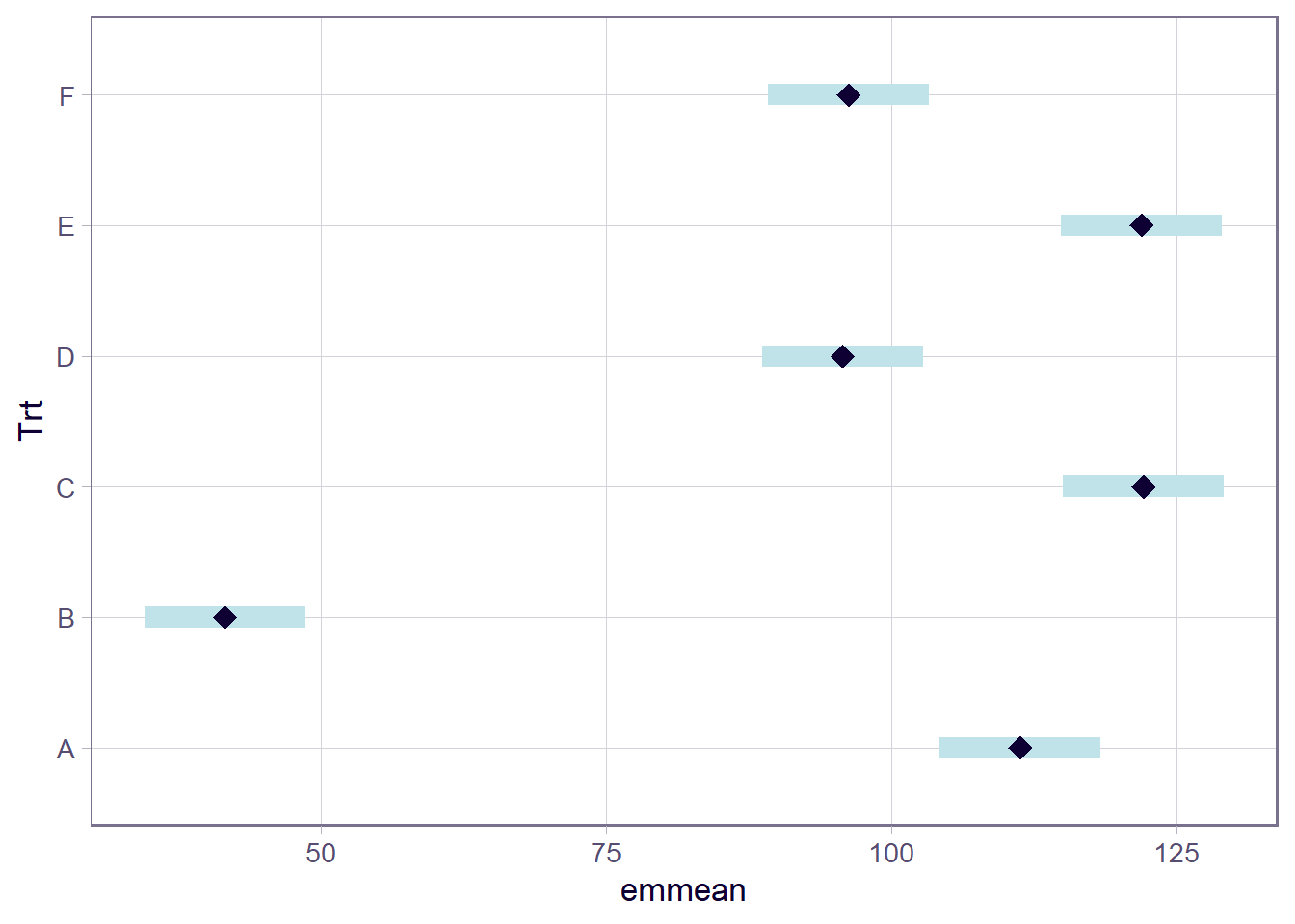
How is the story behind ANOVA and the marginal means so different?
13.2.5 Applied case II – RCBD
- Field experiment studying the effect of potassium on corn yield.
- One treatment factor: Potassium fertilizer (one-way treatment structure).
- Randomized Complete Block Design with 4 repetitions (design structure).
url <- "https://raw.githubusercontent.com/stat720/summer2026/refs/heads/main/data/cochrancox_kfert.csv"

df2 <- read.csv(url) |>
  transmute(K2O_lbac = as.factor(K2O_lbac), rep = as.factor(rep), yield)
Because this is an RCBD, the model is
\[y_{ij} = \mu_0 + T_i + b_j + \varepsilon_{ij}, \\ \varepsilon_{ij} \sim N(0, \sigma^2).\]
Blocks: fixed of random?
- The assumptions behind \(b_j\) vary:
- Fundamentals of mixed models
- Assumption behind blocks as fixed effects: there is a ‘true’ block effect out there.
- Assumption behind blocks as random effects:
- Confidence intervals of the means differ depending on the model:
- Blocks as fixed: \(\hat\mu \pm t \cdot \sqrt{\frac{\sigma_{\varepsilon}^2 }{b}}\)
- Blocks as random: \(\hat\mu \pm t \cdot \sqrt{\frac{\sigma_{\varepsilon}^2 + \sigma^2_{b}}{b}}\)
- Confidence intervals of the means differences don’t differ depending on the model:
- Blocks as fixed/as random: \(\hat\mu \pm t \cdot \sqrt{\frac{2 \sigma_{\varepsilon}^2 }{b}}\)
Blocks as fixed:
m_fixed <- lm(yield ~ K2O_lbac + rep, data = df2)
emmeans(m_fixed, ~ K2O_lbac, contr = list(c(1, -1, 0, 0, 0)))
## $emmeans
## K2O_lbac emmean SE df lower.CL upper.CL
## 36 7.92 0.121 8 7.64 8.19
## 54 8.12 0.121 8 7.84 8.40
## 72 7.81 0.121 8 7.53 8.09
## 108 7.58 0.121 8 7.30 7.86
## 144 7.52 0.121 8 7.24 7.79
##
## Results are averaged over the levels of: rep
## Confidence level used: 0.95
##
## $contrasts
## contrast estimate SE df t.ratio p.value
## c(1, -1, 0, 0, 0) -0.203 0.171 8 -1.191 0.2676
##
## Results are averaged over the levels of: repBlocks as random:
m_random <- lmer(yield ~ K2O_lbac + (1|rep), data = df2)
emmeans(m_random, ~ K2O_lbac, contr = list(c(1, -1, 0, 0, 0)))
## $emmeans
## K2O_lbac emmean SE df lower.CL upper.CL
## 36 7.92 0.162 5.57 7.51 8.32
## 54 8.12 0.162 5.57 7.72 8.52
## 72 7.81 0.162 5.57 7.41 8.21
## 108 7.58 0.162 5.57 7.18 7.98
## 144 7.52 0.162 5.57 7.11 7.92
##
## Degrees-of-freedom method: kenward-roger
## Confidence level used: 0.95
##
## $contrasts
## contrast estimate SE df t.ratio p.value
## c(1, -1, 0, 0, 0) -0.203 0.171 8 -1.191 0.2676
##
## Degrees-of-freedom method: kenward-rogerThings to highlight:
- Under an RCBD, se(mean) \(\neq\) se(mean difference).
- Standard errors of the means differ depending on the model:
- Blocks as fixed: \(\sqrt{\frac{\sigma_{\varepsilon}^2 }{b}}\)
- Blocks as random: \(\sqrt{\frac{\sigma_{\varepsilon}^2 + \sigma^2_{b}}{b}}\)
- Standard errors of the means differences don’t differ depending on the model:
- Blocks as fixed/as random: \(\sqrt{\frac{2 \sigma_{\varepsilon}^2 }{b}}\)
13.3 Applied case III – split-plot design
- Designed experiment of barley (70 levels) with fungicide (2 levels) treatments.
- Two treatment factors: barley (70 levels) and fungicide (2 levels). Two-way factorial treatment structure.
- Split-plot design in an RCBD: Fungicide in the whole plot and genotype in the subplot.
##     yield block gen fung row bed
## 1    5.89    B1 G54   F1   1   1
## 2    6.17    B1 G44   F1   1   2
## 3    5.68    B1 G68   F1   1   3
## 4    5.85    B1 G59   F1   1   4
## 5    5.80    B1 G61   F1   1   5
## 6    6.01    B1 G67   F1   1   6
## 7    5.89    B1 G45   F1   1   7
## 8    4.53    B1 G10   F2   1   8
## 9    5.32    B1 G27   F2   1   9
## 10   5.36    B1 G60   F2   1  10
## 11   5.10    B1 G53   F2   1  11
## 12   5.51    B1 G57   F2   1  12
## 13   5.15    B1 G58   F2   1  13
## 14   5.30    B1 G48   F2   1  14
## 15   5.65    B2 G22   F1   1  15
## 16   5.38    B2 G45   F1   1  16
## 17   5.36    B2 G21   F1   1  17
## 18   5.71    B2 G36   F1   1  18
## 19   5.83    B2 G27   F1   1  19
## 20   5.48    B2 G68   F1   1  20
## 21   5.55    B2 G64   F1   1  21
## 22   4.83    B2 G27   F2   1  22
## 23   4.43    B2 G05   F2   1  23
## 24   4.72    B2 G45   F2   1  24
## 25   4.85    B2 G43   F2   1  25
## 26   5.08    B2 G70   F2   1  26
## 27   4.82    B2 G63   F2   1  27
## 28   4.73    B2 G55   F2   1  28
## 29   5.86    B3 G36   F1   1  29
## 30   5.41    B3 G65   F1   1  30
## 31   5.58    B3 G33   F1   1  31
## 32   5.18    B3 G38   F1   1  32
## 33   5.65    B3 G56   F1   1  33
## 34   5.39    B3 G44   F1   1  34
## 35   5.46    B3 G29   F1   1  35
## 36   4.68    B3 G12   F2   1  36
## 37   4.71    B3 G09   F2   1  37
## 38   4.64    B3 G37   F2   1  38
## 39   4.56    B3 G17   F2   1  39
## 40   4.62    B3 G10   F2   1  40
## 41   4.57    B3 G34   F2   1  41
## 42   4.63    B3 G43   F2   1  42
## 43   4.88    B4 G41   F2   1  43
## 44   4.53    B4 G24   F2   1  44
## 45   5.10    B4 G65   F2   1  45
## 46   4.96    B4 G11   F2   1  46
## 47   5.02    B4 G47   F2   1  47
## 48   4.69    B4 G28   F2   1  48
## 49   5.11    B4 G12   F2   1  49
## 50   5.50    B4 G13   F1   1  50
## 51   4.91    B4 G14   F1   1  51
## 52   5.47    B4 G22   F1   1  52
## 53   5.02    B4 G46   F1   1  53
## 54   5.13    B4 G02   F1   1  54
## 55   5.38    B4 G67   F1   1  55
## 56   5.25    B4 G52   F1   1  56
## 57   6.08    B1 G37   F1   2   1
## 58   6.23    B1 G23   F1   2   2
## 59   6.19    B1 G69   F1   2   3
## 60   5.96    B1 G51   F1   2   4
## 61   5.74    B1 G15   F1   2   5
## 62   5.97    B1 G50   F1   2   6
## 63   5.86    B1 G53   F1   2   7
## 64   5.67    B1 G33   F2   2   8
## 65   5.28    B1 G50   F2   2   9
## 66   5.04    B1 G21   F2   2  10
## 67   5.44    B1 G07   F2   2  11
## 68   5.46    B1 G37   F2   2  12
## 69   5.95    B1 G54   F2   2  13
## 70   4.67    B1 G01   F2   2  14
## 71   5.66    B2 G51   F1   2  15
## 72   5.88    B2 G48   F1   2  16
## 73   4.40    B2 G04   F1   2  17
## 74   5.55    B2 G16   F1   2  18
## 75   5.37    B2 G30   F1   2  19
## 76   5.34    B2 G42   F1   2  20
## 77   5.85    B2 G23   F1   2  21
## 78   4.73    B2 G15   F2   2  22
## 79   5.08    B2 G22   F2   2  23
## 80   5.25    B2 G46   F2   2  24
## 81   5.46    B2 G40   F2   2  25
## 82   5.28    B2 G12   F2   2  26
## 83   5.44    B2 G57   F2   2  27
## 84   4.31    B2 G04   F2   2  28
## 85   5.91    B3 G57   F1   2  29
## 86   5.31    B3 G30   F1   2  30
## 87   5.97    B3 G19   F1   2  31
## 88   5.59    B3 G13   F1   2  32
## 89   6.45    B3 G03   F1   2  33
## 90   5.61    B3 G69   F1   2  34
## 91   5.36    B3 G45   F1   2  35
## 92   4.98    B3 G56   F2   2  36
## 93   4.58    B3 G24   F2   2  37
## 94   4.57    B3 G15   F2   2  38
## 95   5.19    B3 G18   F2   2  39
## 96   4.86    B3 G11   F2   2  40
## 97   5.17    B3 G47   F2   2  41
## 98   4.94    B3 G55   F2   2  42
## 99   5.25    B4 G22   F2   2  43
## 100  4.89    B4 G21   F2   2  44
## 101  5.24    B4 G53   F2   2  45
## 102  5.36    B4 G57   F2   2  46
## 103  5.01    B4 G49   F2   2  47
## 104  4.77    B4 G10   F2   2  48
## 105  4.71    B4 G02   F2   2  49
## 106  5.59    B4 G68   F1   2  50
## 107  5.71    B4 G37   F1   2  51
## 108  5.75    B4 G15   F1   2  52
## 109  5.11    B4 G49   F1   2  53
## 110  5.61    B4 G48   F1   2  54
## 111  5.75    B4 G60   F1   2  55
## 112  5.64    B4 G66   F1   2  56
## 113  5.71    B1 G02   F1   3   1
## 114  6.30    B1 G62   F1   3   2
## 115  5.70    B1 G21   F1   3   3
## 116  5.63    B1 G57   F1   3   4
## 117  5.76    B1 G32   F1   3   5
## 118  5.73    B1 G43   F1   3   6
## 119  5.89    B1 G17   F1   3   7
## 120  4.84    B1 G49   F2   3   8
## 121  4.90    B1 G30   F2   3   9
## 122  5.41    B1 G29   F2   3  10
## 123  5.65    B1 G19   F2   3  11
## 124  5.35    B1 G39   F2   3  12
## 125  5.60    B1 G52   F2   3  13
## 126  5.03    B1 G26   F2   3  14
## 127  5.63    B2 G53   F1   3  15
## 128  5.53    B2 G62   F1   3  16
## 129  6.66    B2 G03   F1   3  17
## 130  5.50    B2 G31   F1   3  18
## 131  5.22    B2 G34   F1   3  19
## 132  5.79    B2 G13   F1   3  20
## 133  5.25    B2 G63   F1   3  21
## 134  4.89    B2 G32   F2   3  22
## 135  4.28    B2 G14   F2   3  23
## 136  4.63    B2 G29   F2   3  24
## 137  4.43    B2 G24   F2   3  25
## 138  4.76    B2 G26   F2   3  26
## 139  5.10    B2 G17   F2   3  27
## 140  5.11    B2 G38   F2   3  28
## 141  5.45    B3 G42   F1   3  29
## 142  5.47    B3 G15   F1   3  30
## 143  5.42    B3 G39   F1   3  31
## 144  5.48    B3 G05   F1   3  32
## 145  5.31    B3 G34   F1   3  33
## 146  5.80    B3 G07   F1   3  34
## 147  5.52    B3 G32   F1   3  35
## 148  4.86    B3 G21   F2   3  36
## 149  5.13    B3 G60   F2   3  37
## 150  4.39    B3 G45   F2   3  38
## 151  5.07    B3 G70   F2   3  39
## 152  4.87    B3 G08   F2   3  40
## 153  5.71    B3 G13   F2   3  41
## 154  4.79    B3 G46   F2   3  42
## 155  5.20    B4 G60   F2   3  43
## 156  4.57    B4 G34   F2   3  44
## 157  5.28    B4 G09   F2   3  45
## 158  5.29    B4 G50   F2   3  46
## 159  5.30    B4 G70   F2   3  47
## 160  5.33    B4 G27   F2   3  48
## 161  5.01    B4 G45   F2   3  49
## 162  5.72    B4 G32   F1   3  50
## 163  5.88    B4 G59   F1   3  51
## 164  5.67    B4 G34   F1   3  52
## 165  5.08    B4 G24   F1   3  53
## 166  5.82    B4 G39   F1   3  54
## [ reached 'max' / getOption("max.print") -- omitted 394 rows ]Because this is a split-plot design, the model is
\[y_{ij} = \mu_0 + F_i + G_j + (F\times G)_{ij} + b_k + wp_{i(k)} + \varepsilon_{ij}, \\ wp_{i(k)}, \sim N(0, \sigma_{wp}^2) \\ \varepsilon_{ij} \sim N(0, \sigma^2_\varepsilon).\]
- Like before, we can choose either fixed or random for \(b_k\).
- But now, the se(mean) depend on the level we are looking.
For differences at the whole-plot level (fung): \(se(\hat\mu-\mu') = \sqrt{\frac{2(\sigma^2_\varepsilon + g \ \sigma^2_{wp})}{b \cdot g}}\). For differences at the split-plot level (gen): \(se(\hat\mu-\mu') = \sqrt{\frac{2(\sigma^2_\varepsilon)}{b \cdot f}}\).
m3 <- lmer(yield ~ gen*fung + (1|block/fung), data = df3)

emmeans(m3, ~fung, contr = list(c(1, -1)))$contr
## contrast estimate SE df t.ratio p.value
## c(1, -1) 0.548 0.0863 3 6.346 0.0079
##
## Results are averaged over the levels of: gen
## Degrees-of-freedom method: kenward-roger## contrast estimate SE df t.ratio p.value
## c(1, -1, 0, 0, 0, 0, 0, 0, 0, 0, 0, 0, 0, 0, 0, 0, 0, 0, 0, 0, -0.152 0.141 414 -1.085 0.2787
##
## Results are averaged over the levels of: fung
## Degrees-of-freedom method: kenward-rogervc <- VarCorr(m3)
sigma2_b <- vc$block[1]
sigma2_wp <- vc$`fung:block`[1]
sigma2_epsilon <- sigma(m3)^2
n_block <- n_distinct(df3$block)
n_fung <- n_distinct(df3$fung)
n_gen <- n_distinct(df3$gen)
#se fung difference
sqrt( 2*(sigma2_epsilon + (n_gen*sigma2_wp)) / (n_block *n_gen) )## [1] 0.086331## [1] 0.1405927