Day 19 Analysis and inference for a split-plot design - Part II

July 8th, 2025

19.1 Announcements

Homework 3 is due this Friday (July 11).
Homework 4 is posted and due next Friday (July 18).
Semester project:
- An example is posted.
- Wednesday July 23: send project for peer review.
- Schedule for somewhere between July 21-August 1 (anywhere between 8am-5pm): 15 min presentation + 15 min Q&A.
- Submit final version of your report by August 1. Include ANOVA, stat model, mock R code, discussion of strengths and weaknesses of the experiment design.

19.2 Review of our experiment

Research question: can we include more banana than the original recipe? Will the optimum temperature change depending on that recipe?
Treatment structure: 3 \(\times\) 2 factorial, with 3 levels for temperature (250, 400, 500) and 2 levels for recipe (Control, Extra Banana)
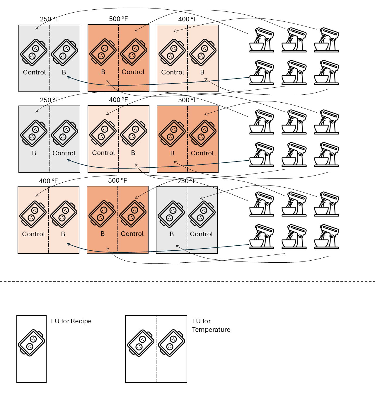
Design structure: split-plot in an CRD, with temperature in the whole plot.

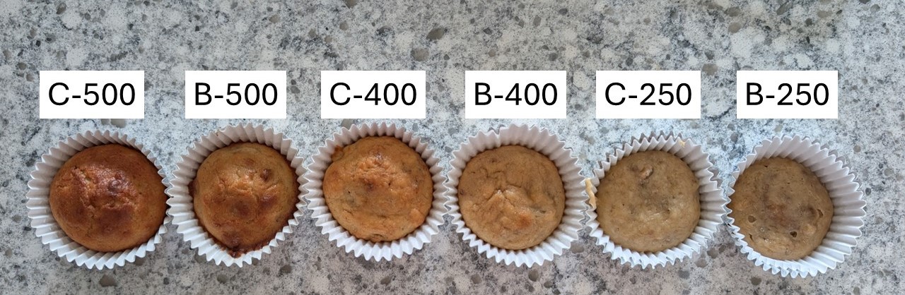
Figure 19.1: Muffin experiment

With that treatment structure, the statistical model will always begin with \(y_{ijk} = \mu + T_i + R_j +(TR)_{ij}\), followed by the effects coming from the design structure (random effects).

19.3 ANOVA tables

19.3.1 Split-plot in a CRD

Table 19.1: ANOVA without subsampling

Table 19.1: Design or Topographical Sources of Variability
Source	df
	-
Error(oven)	t*r-1 = 9-1 = 8
	-
	-
Error(recipe x oven), or recipe(oven)	(b-1)* t * r = (2-1) * 3 * 3 = 9
Total	N-1 = 17

Table 19.1: Treatment Sources of Variability
Source	df
Temperature	t-1 = 3-1 = 2
	-
Banana	b-1 = 2-1 = 1
TxB	(t-1)*(b-1) = 2
Parallels	N-tb = 18 - (3*2) = 12
Total	N-1 = 17

Table 19.1: Combined Table of the Sources of Variability
Source	df
Temperature	t-1 = 3-1 = 2
Error(oven)	t*r-1 - (t-1)= 8 - 2 = 6
Banana	b-1 = 2-1 = 1
TxB	(t-1)*(b-1) = 2
Error(recipe x oven), or recipe(oven)	(b-1)* t * r - (b-1) - (t-1)*(b-1) = 9 - 1 -2 = 6
Total	N-1 = 17

19.3.1.1 Implications on inference

The treatment mean for the \(i\)th temperature and \(j\)th banana level is \(\mu_{ij} = \mu + T_i + B_j +(TB)_{ij}\) and won’t change under different design structures. What may change is the confidence interval around the mean difference.

Recall the formula for a CI: \(\theta \pm t_{df, \frac{\alpha}{2}} \cdot se(\hat{\theta})\).

#get test t
qt(p = .975, df = 6) # df are df error(oven)

## [1] 2.446912

For example, the CI for the differences between means for 250F and 400F \(\mu_{1 \cdot} - \mu_{2 \cdot}\) is \((\mu_{1 \cdot} - \mu_{2 \cdot}) \pm 2.45 \cdot se(\widehat{\mu_{1 \cdot} - \mu_{2 \cdot}})\)
\(se(\widehat{\mu_{1 \cdot} - \mu_{2 \cdot}}) = \sqrt{\frac{2 (\sigma^2_{\varepsilon} + b \cdot \sigma^2_w)}{b \cdot r}}\)

\[\mu_i \pm 2.45 \cdot \sqrt{\frac{2 (\sigma^2_{\varepsilon} + b \cdot \sigma^2_w)}{b \cdot r}}\]

#get test t
qt(p = .975, df = 6) # df are df error(recipe x oven), or recipe(oven)

## [1] 2.446912

The CI for the differences between means for normal and high banana \(\mu_{\cdot 1} - \mu_{\cdot 2}\) is \((\mu_{\cdot 1} - \mu_{\cdot 2}) \pm 2.45 \cdot se(\widehat{\mu_{\cdot 1} - \mu_{\cdot 2}})\)
\(se(\widehat{\mu_{\cdot 1} - \mu_{\cdot 2}}) = \sqrt{\frac{2 \sigma^2_{\varepsilon}}{t \cdot r}}\)

\[\mu_i \pm 2.45 \cdot \sqrt{\frac{2 \sigma^2_{\varepsilon}}{r t}}\]

# libraries
library(tidyverse)
library(lme4)
library(emmeans)

# data
url <- "https://raw.githubusercontent.com/stat720/summer2025/refs/heads/main/data/muffin_data.csv"
muffins <- read.csv(url)
muffins$oven_temp <- as.factor(muffins$oven_temp)
muffins$rep <- as.factor(muffins$rep)
muffins1 <- muffins %>% filter(subsample == 1)

# fit model
model_subsampling <- 
  lmer(height_cm ~ oven_temp*recipe + (1|rep), 
       data = muffins1)

# get variance components
sigma2 <- sigma(model_subsampling)^2
sigma2_r <- 0.1683^2

r <- 3 # nr of repetitions
t <- 3 # nr of levels for temp 
b <- 2 # nr of levels for banana recipe

# see contrast df and SE
emmeans(model_subsampling, ~oven_temp,
        contr = list(c(1, -1, 0)) )

## $emmeans
##  oven_temp emmean    SE df lower.CL upper.CL
##  250         2.30 0.152  6     1.93     2.67
##  400         2.62 0.152  6     2.24     2.99
##  500         3.02 0.152  6     2.64     3.39
## 
## Results are averaged over the levels of: recipe 
## Degrees-of-freedom method: kenward-roger 
## Confidence level used: 0.95 
## 
## $contrasts
##  contrast    estimate    SE df t.ratio p.value
##  c(1, -1, 0)   -0.317 0.216  6  -1.469  0.1923
## 
## Results are averaged over the levels of: recipe 
## Degrees-of-freedom method: kenward-roger

# this should match the SE above
sqrt(2*(sigma2 + b*sigma2_r)/(r*b))

## [1] 0.2155826

# see contrast df and SE
emmeans(model_subsampling, ~recipe,
        contr = list(c(1, -1)) )

## $emmeans
##  recipe emmean    SE   df lower.CL upper.CL
##  B        2.30 0.111 11.3     2.06     2.54
##  C        2.99 0.111 11.3     2.75     3.23
## 
## Results are averaged over the levels of: oven_temp 
## Degrees-of-freedom method: kenward-roger 
## Confidence level used: 0.95 
## 
## $contrasts
##  contrast estimate    SE df t.ratio p.value
##  c(1, -1)   -0.689 0.136  6  -5.079  0.0023
## 
## Results are averaged over the levels of: oven_temp 
## Degrees-of-freedom method: kenward-roger

# this should match the SE above
sqrt(2*sigma2/(r*t))

## [1] 0.1356284

19.3.2 Same design as above, with subsampling

Table 19.2: ANOVA without subsampling

Table 19.2: Design or Topographical Sources of Variability
Source	df
	-
Error(oven)	t*r-1 = 9-1 = 8
	-
	-
Error(recipe x oven), or recipe(oven)	(b-1)* t * r = (2-1) * 3 * 3 = 9
Error(muffin x recipe x oven), or muffin(recipe x oven)	(s-1)* b * t * r = (3-1) * 2 * 3 * 3 = 36
Total	N-1 = 53

Table 19.2: Treatment Sources of Variability
Source	df
Temperature	t-1 = 3-1 = 2
	-
Banana	b-1 = 2-1 = 1
TxB	(t-1)*(b-1) = 2
Parallels	N-tb = 54 - (3*2) = 48
Total	N-1 = 53

Table 19.2: Combined Table of the Sources of Variability
Source	df
Temperature	t-1 = 3-1 = 2
Error(oven)	t*r-1 - (t-1)= 8 - 2 = 6
Banana	b-1 = 2-1 = 1
TxB	(t-1)*(b-1) = 2
Error(recipe x oven), or recipe(oven)	(b-1)* t * r - (b-1) - (t-1)*(b-1) = 9 - 1 -2 = 6
Error(muffin x recipe x oven), or muffin(recipe x oven)	(s-1)* b * t * r = 36
Total	N-1 = 53

19.4 Applied analysis in R

Get code here.