Day 17 Analyzing data from a split-plot design
July 3rd, 2025
17.1 Announcements
- Planning to miss >2 classes in July? survey
- Watch last week’s classes (especially days 3+4)
- Homework 3 is posted and due next Friday (July 11).
17.2 Background
We designed an experiment a split-plot design to figure out the best temperature and recipe to bake the muffins. Check out the original recipe here.
An appropriate model to describe the data is:
\[y_{ijk} = \mu + T_i + R_j + (TR)_{ij} + b_k + w_{i(k)} + \varepsilon_{ijk},\]
\[b_k \sim N(0, \sigma_b^2), \\w_{i(k)} \sim N(0, \sigma^2_w), \\ \varepsilon_{ijk} \sim N(0, \sigma_{\varepsilon}^2).\]
17.2.1 Research question
What is the best temperature to bake the muffins?
- 250 °F
- 400 °F
- 500 °F
How much banana?
- 1 1/2 cups (12.75 oz, or 361 gr.)
- 2 cups (17 oz, or 482 gr.)
|
|
|
|
|
|
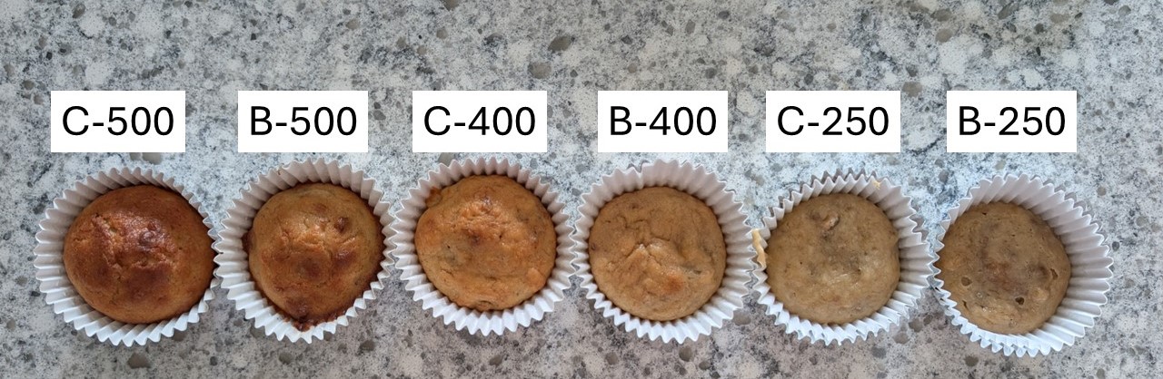
Figure 17.1: Muffin experiment
17.3 Analyzing the data
Get code here.
17.4 Treatment means and confidence intervals for the split-plot design
The treatment mean for the \(i\)th temperature and \(j\)th banana level is \(\mu_{ij} = \mu + T_i + B_j +(TB)_{ij}\). That mean won’t change under different design structures. What may change is the confidence interval around the mean difference.
- First, recall the formula for a CI: \(\theta \pm t_{df, \frac{\alpha}{2}} \cdot se(\hat{\theta})\)
## [1] 2.776445- For example, the CI for the differences between means for 300F and 400F \(\mu_{1 \cdot} - \mu_{2 \cdot}\) is \((\mu_{1 \cdot} - \mu_{2 \cdot}) \pm 2.78 \cdot se(\widehat{\mu_{1 \cdot} - \mu_{2 \cdot}})\)
- \(se(\widehat{\mu_{1 \cdot} - \mu_{2 \cdot}}) = \sqrt{\frac{2 (\sigma^2_{\varepsilon} + b \cdot \sigma^2_w)}{b \cdot r}}\)
\[\mu_i \pm 2.78 \cdot \sqrt{\frac{2 (\sigma^2_{\varepsilon} + b \cdot \sigma^2_w)}{b \cdot r}}\]
## [1] 2.446912- The CI for the differences between means for normal and high banana \(\mu_{\cdot 1} - \mu_{\cdot 2}\) is \((\mu_{\cdot 1} - \mu_{\cdot 2}) \pm 2.44 \cdot se(\widehat{\mu_{\cdot 1} - \mu_{\cdot 2}})\)
- \(se(\widehat{\mu_{\cdot 1} - \mu_{\cdot 2}}) = \sqrt{\frac{2 \sigma^2_{\varepsilon}}{t \cdot r}}\)
\[\mu_i \pm 2.44 \cdot \sqrt{\frac{2 \sigma^2_{\varepsilon}}{r}}\]