Day 26 Planning a multi-location design
July 17th, 2025
26.2 Planning a multi-environment trial
- Objectives:
- Cover more variability in the target environment
- Increase number of repetitions
- Different approaches to picking the multiple locations:
- Carefully select multiple environments
- Randomly(ish) select multiple environments within the target environment
- How do both affect the response?
26.2.2 What do the results for different multi-environment trials look like?
Below is a simulation comparing 3 different scenarios of multi-environment trials with different number of environments tested. We assume that, within each environment, the trial is an RCBD with three repetitions. [Context: this is perhaps the most common design in agronomy.]
We assume the following data generating process: \[y_{ijk} = \mu_i + b_{j(k)} + u_k +\varepsilon_{ijk}, \\ b_{j(k)} \sim N(0, \sigma_{b}^2), \\ u_k \sim N(0, \sigma_{u}^2), \\ \varepsilon_{ijk} \sim N(0, \sigma_{\varepsilon}^2),\] where:
- \(\mu_i\) is the treatment mean for the \(i\)th treatment (\(i = 1,2, ..., 30\)),
- \(b_{j(k)}\) is the effect of the \(j\)th block in the \(k\)th environment (\(j = 1,2,3\)),
- \(u_k\) is the effect of the \(k\)th environment (\(k = 1,2,..., E\)), and
- \(\varepsilon_{ijk}\) is the residual for the observation corresponding to the \(i\)th treatment, \(j\)th block in the \(k\)th environment.
For this simulation, we assume that all \(b_{j(k)}\), \(u_k\) and \(\varepsilon_{ijk}\) arise from independent normal distributions, with variances \(\sigma_{b}^2 = 3\), \(\sigma_{u}^2 = 35\), \(\sigma_{\varepsilon}^2 = 10\).
Each simulation consists of 3 steps:
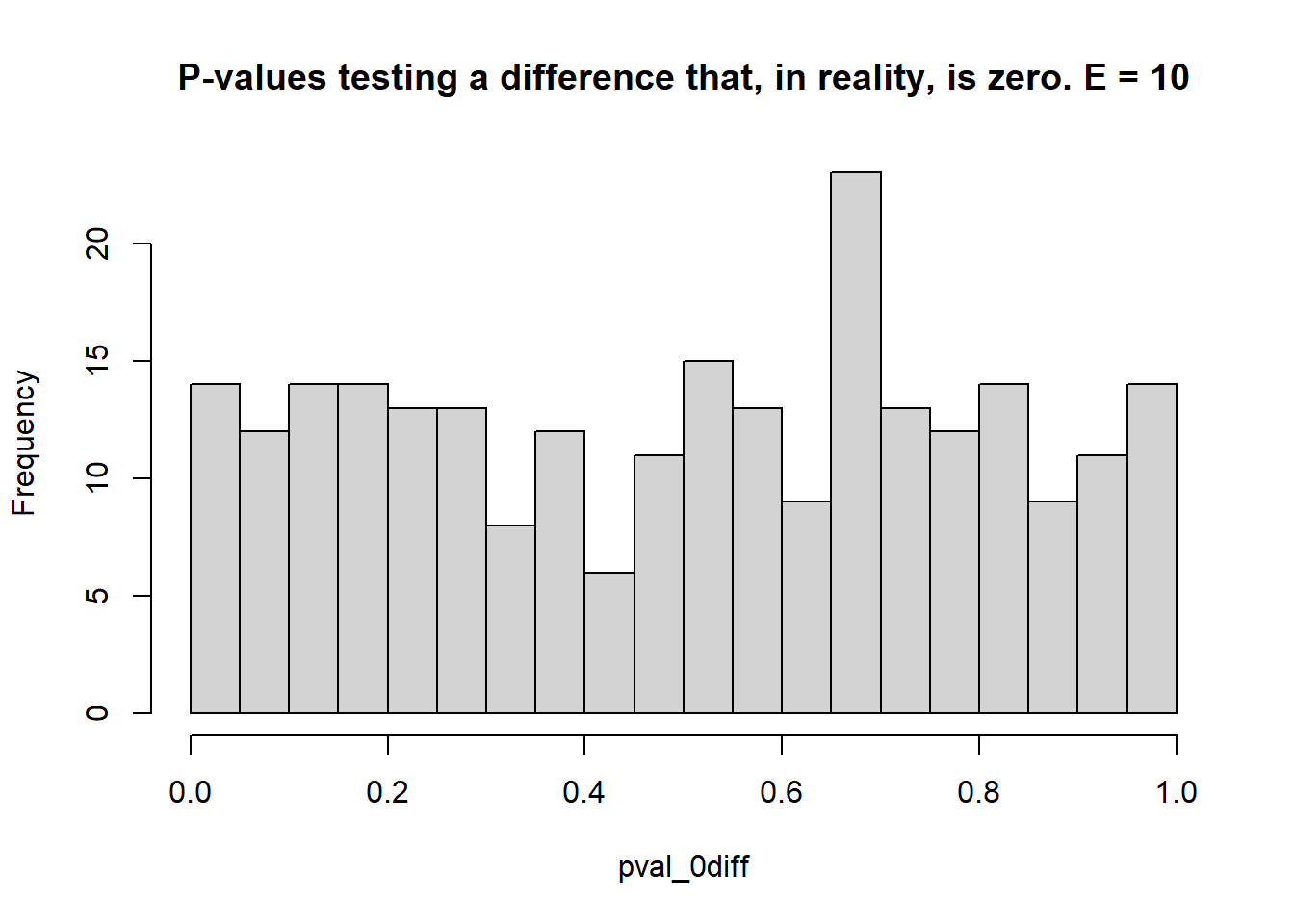
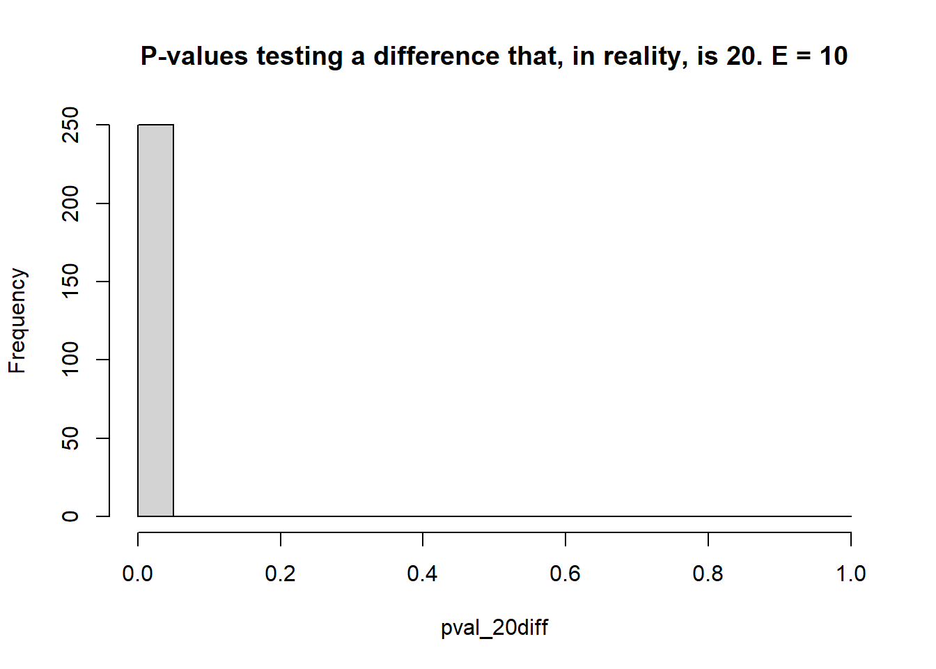
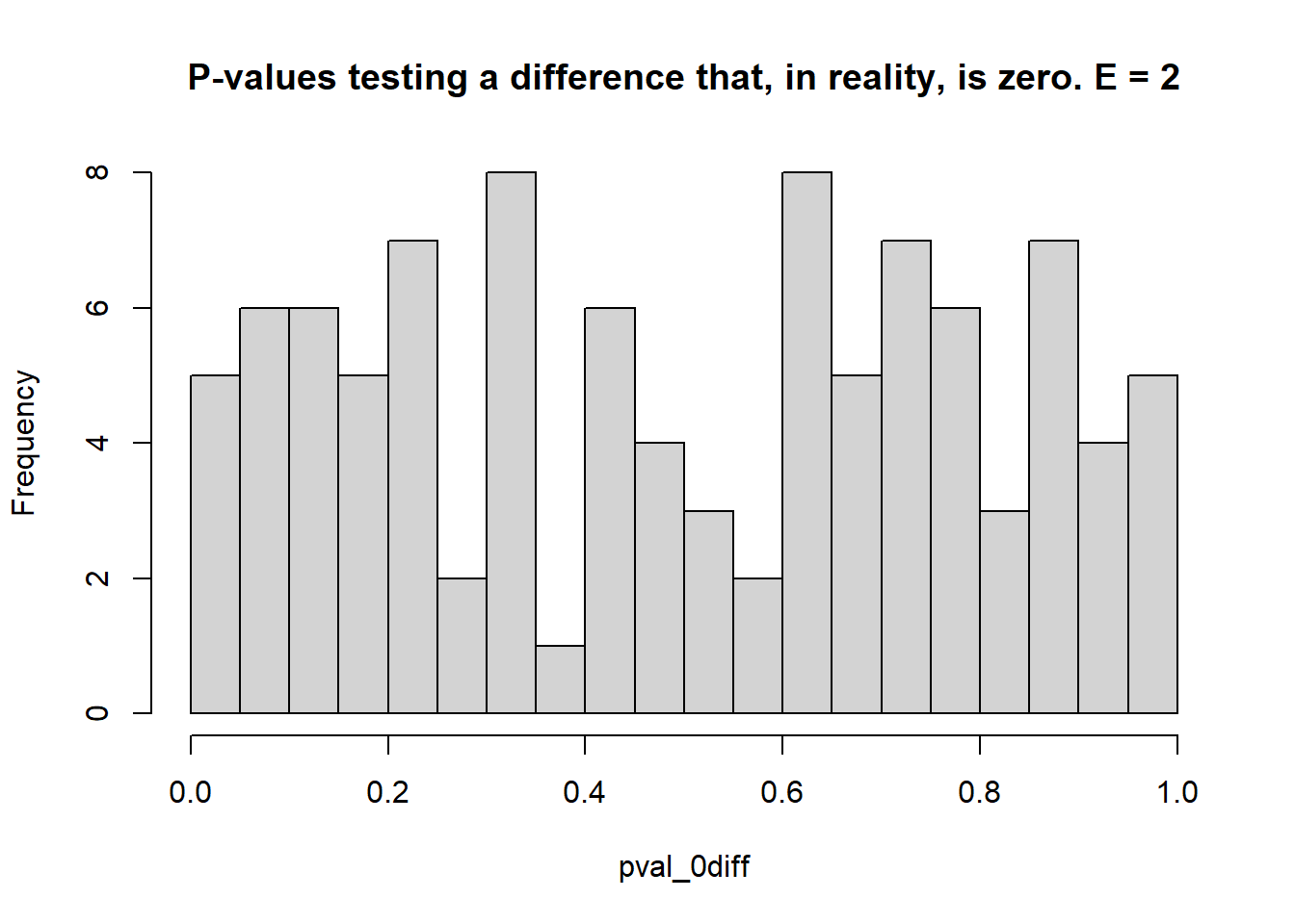
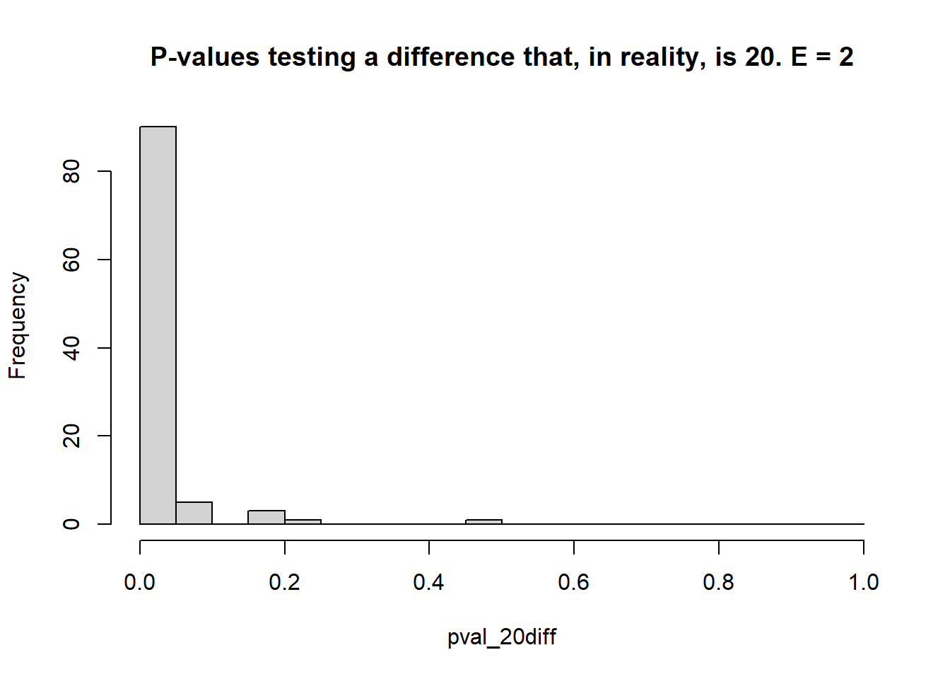
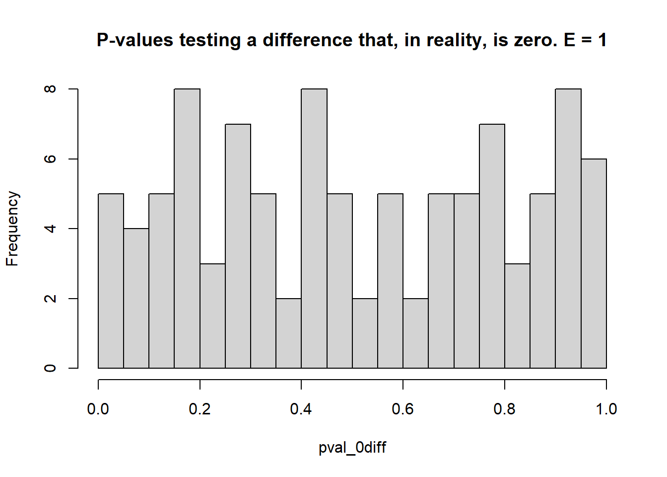
- Set “true” states (i.e., set \(\mu_i\)). We assume the same “ground truth” for all cases. To demonstrate the properties of the designs, we will assume some treatments have no difference (i.e., \(\mu_i = \mu_{i'}\)) and others are different (i.e., \(\mu_i \neq \mu_{i'}\)). Note: this step does not depend on sample size.
- Draw random samples from \(b_{j(k)}\), \(u_k\) and \(\varepsilon_{ijk}\) to simulate observed values \(y_{ijk}\). Note: this step depends on sample size.
- Estimate the \(\mu_i\)s and test the type I error rate (count of times when \(p<0.05\) when the truth was actually \(\mu_i = \mu_{i'}\) – reject \(H_0\) when it was true), and the statistical power (count of times when \(p<0.05\) when the truth was \(\mu_i \ne \mu_{i'}\) – reject \(H_0\) when it was false).
R packages required for this simulation
library(tidyverse) # data wrangling & data viz
library(lme4) # model fitting
library(emmeans) # marginal means
Simulate 100 hypothetical experiments for 3 scenarios:
- 10 environments, 3 blocks each
Click to show code for the simulation
sigma_env.truth <- 35
sigma_block.truth <- 3
sigma.truth <- 10

trts <- paste("t", 11:40, sep = "")
n_envs <- 10
n_rep <- 3
n_sims <- 250

df_me <- expand.grid(trt = trts,
                     rep = 1:n_rep,
                     environm = paste("e", 11:(10+n_envs), sep = ""))

pval_0diff <- numeric(n_sims)
pval_20diff <- numeric(n_sims)

for (i in 1:n_sims) {
  env_re <- rnorm(n_envs, 0, sigma_env.truth)
  block_re <- rnorm(n_envs*n_rep, 0, sigma_block.truth)

  df_envs <- data.frame(environm = paste("e", 11:(10+n_envs), sep = ""),
                        env_re)
  df_blocks <- expand.grid(environm = paste("e", 11:(10+n_envs), sep = ""),
                           rep = 1:n_rep) %>%
    mutate(block_re = block_re)

  df_me <- df_me %>%
    mutate(mu_t = case_when(trt == "t11" ~ 200,
                            trt == "t12" ~ 200,
                            trt == "t13" ~ 180,
                            .default = 220)) %>%
    left_join(df_envs) %>%
    left_join(df_blocks) %>%
    mutate(e = rnorm(nrow(df_me), 0, sigma.truth),
           y = mu_t + env_re + block_re + e)


  m <- lmer(y ~ trt + (1|environm/rep), data = df_me)
  pval_0diff[i] <- as.data.frame(emmeans(m, ~ trt, contr = list(c(1, -1, rep(0, 28))))$contr)$p.value
  pval_20diff[i] <- as.data.frame(emmeans(m, ~ trt, contr = list(c(1, 0, 0, -1, rep(0, 26))))$contr)$p.value
} 
## [1] 0.056## [1] 1- 2 environments, 3 blocks each
Click to show code for the simulation
sigma_env.truth <- 35
sigma_block.truth <- 3
sigma.truth <- 10

trts <- paste("t", 11:40, sep = "")
n_envs <- 2
n_rep <- 3
n_sims <- 100

df_me <- expand.grid(trt = trts,
                     rep = 1:n_rep,
                     environm = paste("e", 11:(10+n_envs), sep = ""))

pval_0diff <- numeric(n_sims)
pval_20diff <- numeric(n_sims)

set.seed(3)
for (i in 1:n_sims) {
  env_re <- rnorm(n_envs, 0, sigma_env.truth)
  block_re <- rnorm(n_envs*n_rep, 0, sigma_block.truth)

  df_envs <- data.frame(environm = paste("e", 11:(10+n_envs), sep = ""),
                        env_re)
  df_blocks <- expand.grid(environm = paste("e", 11:(10+n_envs), sep = ""),
                           rep = 1:n_rep) %>%
    mutate(block_re = block_re)

  df_me <- df_me %>%
    mutate(mu_t = case_when(trt == "t11" ~ 200,
                            trt == "t12" ~ 200,
                            trt == "t13" ~ 180,
                            .default = 220)) %>%
    left_join(df_envs) %>%
    left_join(df_blocks) %>%
    mutate(e = rnorm(nrow(df_me), 0, sigma.truth),
           y = mu_t + env_re + block_re + e)


  m <- lmer(y ~ trt + (1|environm/rep), data = df_me)
  pval_0diff[i] <- as.data.frame(emmeans(m, ~ trt, contr = list(c(1, -1, rep(0, 28))))$contr)$p.value
  pval_20diff[i] <- as.data.frame(emmeans(m, ~ trt, contr = list(c(1, 0, 0, -1, rep(0, 26))))$contr)$p.value
}
## [1] 0.05## [1] 0.9- 1 environment, 3 blocks each
Click to show code for the simulation
sigma_env.truth <- 35
sigma_block.truth <- 3
sigma.truth <- 10

trts <- paste("t", 11:40, sep = "")
n_envs <- 1
n_rep <- 3
n_sims <- 100

df_me <- expand.grid(trt = trts,
                     rep = 1:n_rep,
                     environm = paste("e", 11:(10+n_envs), sep = ""))

pval_0diff <- numeric(n_sims)
pval_20diff <- numeric(n_sims)

set.seed(3)
for (i in 1:n_sims) {
  env_re <- rnorm(n_envs, 0, sigma_env.truth)
  block_re <- rnorm(n_envs*n_rep, 0, sigma_block.truth)

  df_envs <- data.frame(environm = paste("e", 11:(10+n_envs), sep = ""),
                        env_re)
  df_blocks <- expand.grid(environm = paste("e", 11:(10+n_envs), sep = ""),
                           rep = 1:n_rep) %>%
    mutate(block_re = block_re)

  df_me <- df_me %>%
    mutate(mu_t = case_when(trt == "t11" ~ 200,
                            trt == "t12" ~ 200,
                            trt == "t13" ~ 180,
                            .default = 220)) %>%
    left_join(df_envs) %>%
    left_join(df_blocks) %>%
    mutate(e = rnorm(nrow(df_me), 0, sigma.truth),
           y = mu_t + env_re + block_re + e)


  m <- lmer(y ~ trt + (1|rep), data = df_me)
  pval_0diff[i] <- as.data.frame(emmeans(m, ~ trt, contr = list(c(1, -1, rep(0, 28))))$contr)$p.value
  pval_20diff[i] <- as.data.frame(emmeans(m, ~ trt, contr = list(c(1, 0, 0, -1, rep(0, 26))))$contr)$p.value
}
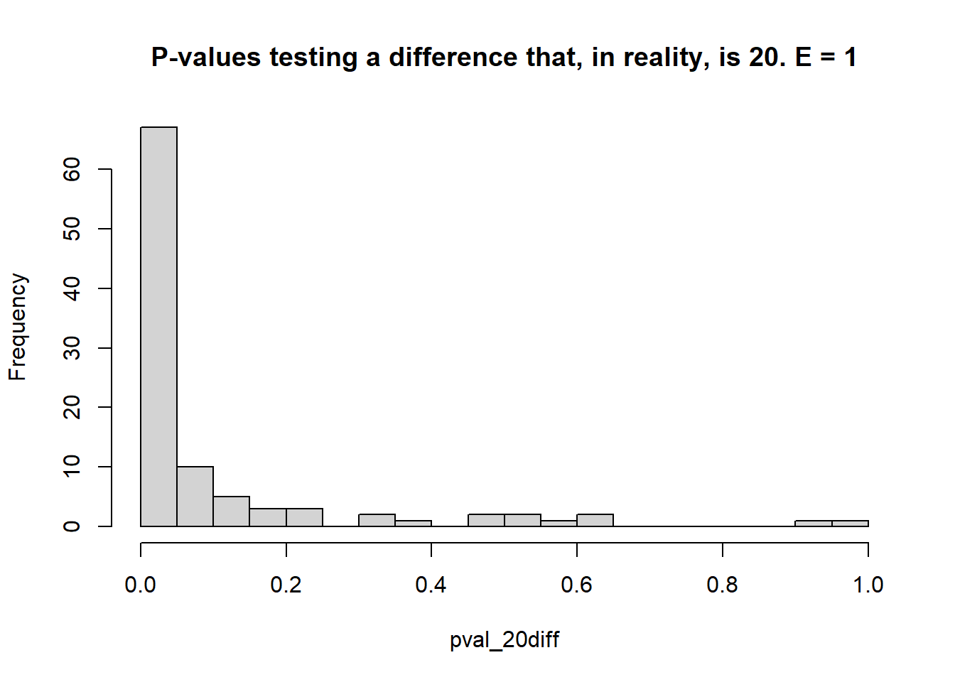
## [1] 0.05## [1] 0.67