Day 3 Basic types of designed experiments
June 11th, 2025
3.1 Review
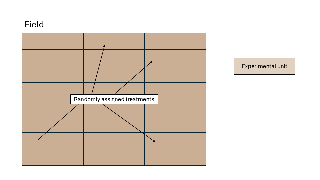
- Experimental unit
- The golden rules of designed experiments:
- Replication
- Randomization
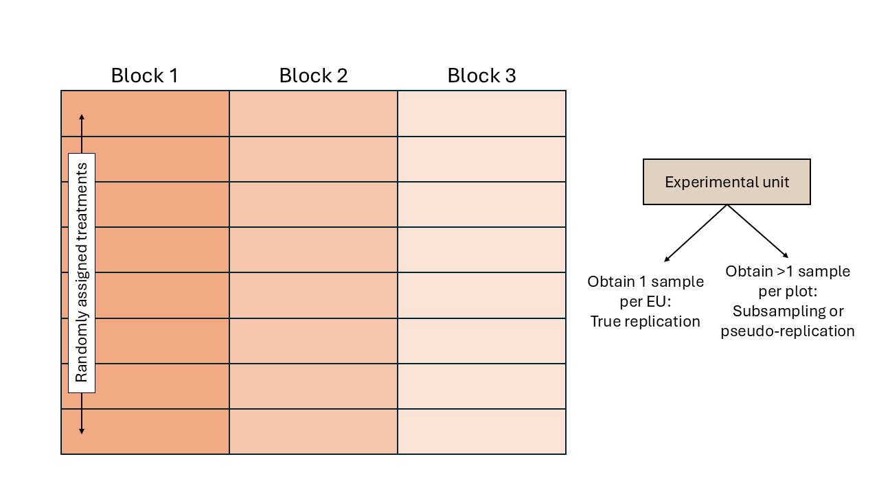
- Local control (blocking)
3.2 Types of designs
3.3 Building an ANOVA skeleton using design (aka topographical) and treatment elements
|
|
|
This way to do an ANOVA is normally considered the “What Would Fisher Do” ANOVA. Sir R.A. Fisher did plenty of his very influential work while he was working at the Rothamsted Agricultural Station!
3.4 Linear model good old friend
- What does “linear” mean?
- What does “ANOVA” mean?
\[\begin{equation} y_{ij} = \mu + \tau_i + \varepsilon_{ij}, \\ \varepsilon_{ij} \sim N(0, \sigma^2), \end{equation}\]
OR
\[\begin{equation} y_{i} = \beta_0 + x_{1i}\beta_1 +x_{2i}\beta_2 + x_{3i}\beta_3 + \varepsilon_{i}, \\ \varepsilon_{i} \sim N(0, \sigma^2), \\ x_{1i} = \begin{cases} 1, & \text{if treatment A}\\ 0, & \text{otherwise} \end{cases} \\ x_{2i} = \begin{cases} 1, & \text{if treatment B}\\ 0, & \text{otherwise} \end{cases} \\ x_{3i} = \begin{cases} 1, & \text{if treatment C}\\ 0, & \text{otherwise} \end{cases} \end{equation}\]
OR
\[\begin{equation} \mathbf{y} = \mathbf{X}\boldsymbol{\beta} + \boldsymbol{\varepsilon}, \\ \boldsymbol{\varepsilon} \sim N(\boldsymbol{0}, \sigma^2 \mathbf{I}), \\ \end{equation}\]
OR
\[\begin{equation} \mathbf{y} \sim N(\boldsymbol{\mu}, \sigma^2 \mathbf{I}), \\ \boldsymbol{\mu} = \mathbf{X}\boldsymbol{\beta} + \boldsymbol{\varepsilon} \end{equation}\]
3.4.1 The most common assumptions behind most software
- Constant variance
- Independence
- Normality
We can describe the general linear model as \[\begin{equation} y_{ij} = \mu + \tau_i + \varepsilon_{ij}, \end{equation}\] \[\begin{equation} \varepsilon_{ij} \sim N(0, \sigma^2), \end{equation}\] where \(y_{ij}\) is the \(j\)th observation of the \(i\)th treatment, \(\mu\) is the overall mean, \(\tau_i\) is the treatment effect of the \(i\)th treatment, and \(\varepsilon_{ij}\) is the residual for the \(j\)th observation of the \(i\)th treatment (i.e., the difference between observed and predicted).
The form used to describe the model above is called “Model equation form”.
Another way of saying the same is the “Probability distribution form”, where we describe the distribution of \(y\) directly.
\[\begin{equation}
y_{ij} \sim N(\mu_{ij}, \sigma^2),
\end{equation}\]
or
\[\begin{equation}
\mathbf{y} \sim N(\mu_{ij}, \sigma^2).
\end{equation}\]
3.5 Some Practice
Check out this R script to follow along!