Day 23 Randomized complete block designs
July 14th, 2025
23.1 Announcements
- HW 4 due Friday
- Topics for the week of July 21 - survey
23.2 Randomized complete block designs
- Blocks are groups of approximately similar experimental units.
- Data generated by blocked designs may be analyzed as \(y_{ij} = \mu +\tau_i + b_j + \varepsilon_{ij}\), where \(y_{ij}\) is the observed response for the \(i\)th treatment in the \(j\)th block, \(\tau_i\) is the effect of the \(i\)th treatment (\(i = 1, 2, ..., t\)), \(b_j\) is the effect of the \(j\)th block, \(\varepsilon_{ij}\) is the residual of the \(i\)th treatment in the \(j\)th block.
- Most RCBDs have \(k = t\), where \(k\) is the number of experimental units per block, and \(t\) is the number of treatments.
23.3 Blocks - fixed or random?
- The assumptions behind \(b_j\) vary:
- Fundamentals of mixed models
- Assumption behind blocks as fixed effects: there is a ‘true’ block effect out there.
- Assumption behind blocks as random effects:
- Confidence intervals of the means differ depending on the model:
- Blocks as fixed: \(\hat\mu \pm t \cdot \sqrt{\frac{\sigma_{\varepsilon}^2 }{b}}\)
- Blocks as random: \(\hat\mu \pm t \cdot \sqrt{\frac{\sigma_{\varepsilon}^2 + \sigma^2_{b}}{b}}\)
- Confidence intervals of the means differences don’t differ depending on the model:
- Blocks as fixed/as random: \(\hat\mu \pm t \cdot \sqrt{\frac{2 \sigma_{\varepsilon}^2 }{b}}\)
- Blocks as fixed/as random: \(\hat\mu \pm t \cdot \sqrt{\frac{2 \sigma_{\varepsilon}^2 }{b}}\)
- More on the differences between blocks as fixed vs random: Dixon 2016.
23.3.1 Applied design and analysis of an RCBD
An experiment was run in South Australia to compare for 107 different wheat varieties, in a randomized complete block design with 3 blocks.
Get R code here.
| Source | df |
|---|---|
| Blocks | b-1 = 2 |
| Genotype | g-1 = 106 |
| Error | N-b-g+1 = 221 |
| Total | N-1 = 329 |
library(tidyverse)
library(agridat)
library(lme4)
library(emmeans)

dat_wheat_rcbd <- agridat::gilmour.serpentine

dat_wheat_rcbd %>%
  ggplot(aes(col, row))+
  geom_tile(aes(fill = rep))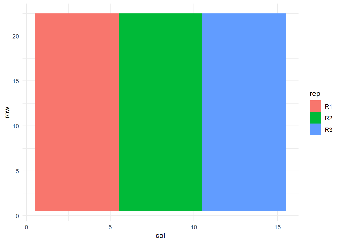
m_block.as.fixed <- lm(yield ~ gen + rep, data = dat_wheat_rcbd)

m_block.as.random <- lme4::lmer(yield ~ gen + (1|rep), data = dat_wheat_rcbd)

emmeans(m_block.as.fixed, ~gen)[1:10,]
## gen emmean SE df lower.CL upper.CL
## (WWH*MM)*WR* 709 66.7 221 577 841
## (WqKPWmH*3Ag 733 66.7 221 602 865
## AMERY 616 66.7 221 484 747
## ANGAS 576 66.7 221 445 708
## AROONA 555 66.7 221 424 687
## BATAVIA 534 66.7 221 402 665
## BD231 639 66.7 221 507 770
## BEULAH 535 66.7 221 404 667
## BLADE 439 66.7 221 307 571
## BT_SCHOMBURG 660 66.7 221 528 792
##
## Results are averaged over the levels of: rep
## Confidence level used: 0.95## gen emmean SE df lower.CL upper.CL
## (WWH*MM)*WR* 709 93.3 8.16 495 923
## (WqKPWmH*3Ag 733 93.3 8.16 519 948
## AMERY 616 93.3 8.16 401 830
## ANGAS 576 93.3 8.16 362 791
## AROONA 555 93.3 8.16 341 770
## BATAVIA 534 93.3 8.16 319 748
## BD231 639 93.3 8.16 424 853
## BEULAH 535 93.3 8.16 321 750
## BLADE 439 93.3 8.16 225 653
## BT_SCHOMBURG 660 93.3 8.16 446 874
##
## Degrees-of-freedom method: kenward-roger
## Confidence level used: 0.95emmeans(m_block.as.fixed, ~gen, contr = list(c(1, -1, rep(0, n_distinct(dat_wheat_rcbd$gen)-2))))$contr## contrast estimate SE df t.ratio p.value
## c(1, -1, 0, 0, 0, 0, 0, 0, 0, 0, 0, 0, 0, 0, 0, 0, 0, 0, 0, 0, -24.3 94.4 221 -0.258 0.7968
##
## Results are averaged over the levels of: repemmeans(m_block.as.random, ~gen, contr = list(c(1, -1, rep(0, n_distinct(dat_wheat_rcbd$gen)-2))))$contr## contrast estimate SE df t.ratio p.value
## c(1, -1, 0, 0, 0, 0, 0, 0, 0, 0, 0, 0, 0, 0, 0, 0, 0, 0, 0, 0, -24.3 94.4 221 -0.258 0.7968
##
## Degrees-of-freedom method: kenward-rogerbind_rows(as.data.frame(emmeans(m_block.as.fixed, ~gen)[1:10,]) %>% transmute(gen, emmean, SE, blocks = "fixed"),
as.data.frame(emmeans(m_block.as.random, ~gen)[1:10,]) %>% transmute(gen, emmean, SE, blocks = "random")) %>%
ggplot(aes(gen, emmean))+
geom_errorbar(aes(ymin = emmean - SE, ymax = emmean + SE, color = blocks), width = .1, position = position_dodge(.1))+
geom_point()+
scale_color_manual(values = c("tomato", "#1282A2"))+
theme(axis.text = element_text(angle = 30))+
labs(title = "Difference in Mean SE between fixed blocks and random blocks analyses")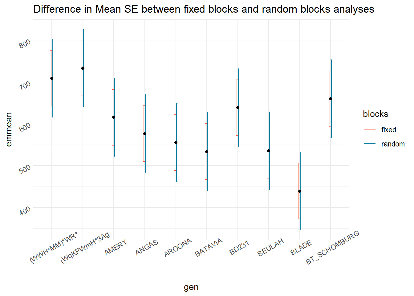
bind_rows(as.data.frame(emmeans(m_block.as.fixed, ~gen, contr = list(c(1, -1, rep(0, n_distinct(dat_wheat_rcbd$gen)-2)),
                                                                     c(1, 0, -1, rep(0, n_distinct(dat_wheat_rcbd$gen)-3))))$contr) %>%
            transmute(estimate, SE, blocks = "fixed", contrast = c("t1 vs. t2", "t1 vs. t3")),
          as.data.frame(emmeans(m_block.as.random, ~gen, contr = list(c(1, -1, rep(0, n_distinct(dat_wheat_rcbd$gen)-2)),
                                                                     c(1, 0, -1, rep(0, n_distinct(dat_wheat_rcbd$gen)-3))))$contr) %>%
            transmute(estimate, SE, blocks = "random", contrast = c("t1 vs. t2", "t1 vs. t3"))) %>%
  ggplot(aes(contrast, estimate))+
  geom_errorbar(aes(ymin = estimate - SE, ymax = estimate + SE, color = blocks), width = 0.05, position = position_dodge(.05))+
  geom_point()+
  scale_color_manual(values = c("tomato", "#1282A2"))+
  theme(axis.text = element_text(angle = 30))+
  labs(title = "Difference in Contrast SE between fixed blocks and random blocks analyses")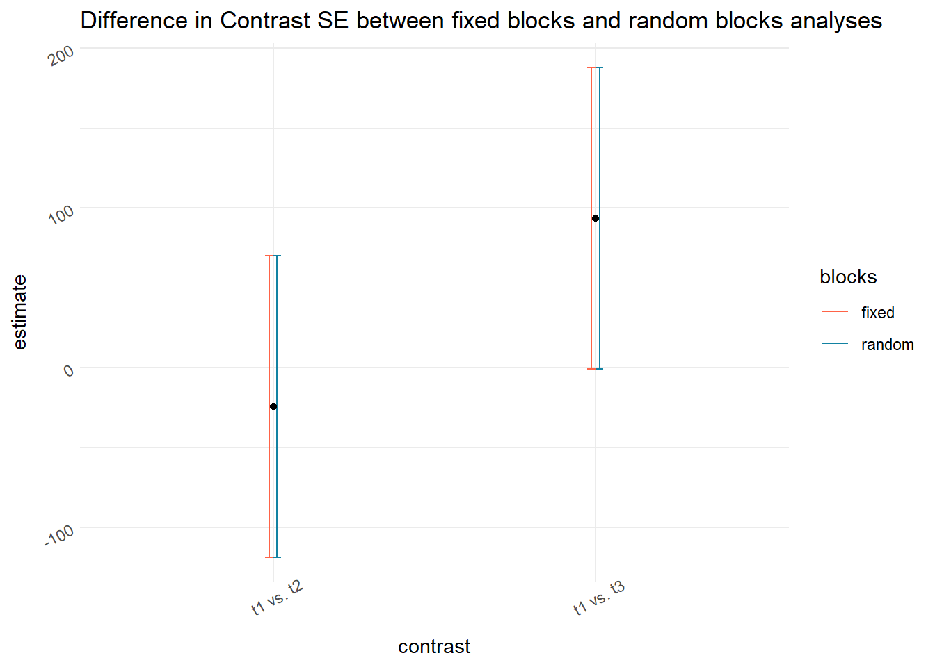
Mean standard error, blocks as fixed: \(\sqrt{\frac{\sigma_{\varepsilon}^2 }{b}}\)
n_blocks <- n_distinct(dat_wheat_rcbd$rep)
sigma2_blocks.as.fixed <- sigma(m_block.as.fixed)^2

sqrt(sigma2_blocks.as.fixed / n_blocks)
## [1] 66.73095Blocks as random: \(\hat\mu \pm t \cdot \sqrt{\frac{\sigma_{\varepsilon}^2 + \sigma^2_{b}}{b}}\)
sigma2_blocks.as.random <- sigma(m_block.as.random)^2
sigma2b_blocks.as.random <- as.data.frame(VarCorr(m_block.as.random))[1, 'sdcor']^2

sqrt((sigma2b_blocks.as.random + sigma2_blocks.as.random) / n_blocks)
## [1] 93.2654923.4 Incomplete block designs
- Same model as before: \(y_{ij} = \mu +\tau_i + b_j + \varepsilon_{ij}\), where \(y_{ij}\) is the observed response for the \(i\)th treatment in the \(j\)th block, \(\tau_i\) is the effect of the \(i\)th treatment (\(i = 1, 2, ..., t\)), \(b_j\) is the effect of the \(j\)th block, \(\varepsilon_{ij}\) is the residual of the \(i\)th treatment in the \(j\)th block.
- In IBDs, \(k < t\), where \(k\) is the number of experimental units per block, and \(t\) is the number of treatments.
- Better interblock information recovery with random \(b_j\).
23.4.1 Applied design and analysis of a Balanced IBD
The data below correspond to a study comparing soybean genotypes in a balanced incomplete block designed experiment.
| Source | df |
|---|---|
| Blocks | b-1 = 30 |
| Genotype | g-1 = 30 |
| Error | N-b-g+1 = 125 |
| Total | N-1 = 185 |
dat_soy_ibd <- agridat::weiss.incblock

dat_soy_ibd %>%
  ggplot(aes(col, row))+
  geom_tile(aes(fill = block))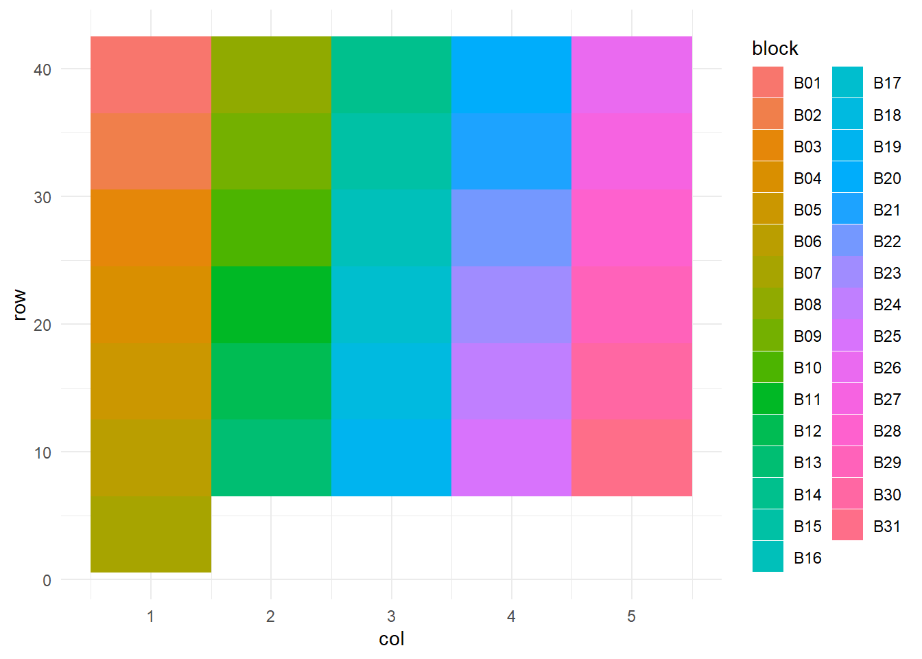
m_block.as.fixed <- lm(yield ~ gen + block, data = dat_soy_ibd)

m_block.as.random <- lme4::lmer(yield ~ gen + (1|block), data = dat_soy_ibd)

emmeans(m_block.as.fixed, ~gen)[1:10,]
## gen emmean SE df lower.CL upper.CL
## G01 24.6 0.831 125 22.9 26.2
## G02 26.9 0.831 125 25.3 28.6
## G03 32.6 0.831 125 31.0 34.3
## G04 27.0 0.831 125 25.3 28.6
## G05 26.0 0.831 125 24.4 27.7
## G06 32.0 0.831 125 30.3 33.6
## G07 24.2 0.831 125 22.5 25.8
## G08 27.6 0.831 125 26.0 29.3
## G09 29.3 0.831 125 27.6 30.9
## G10 24.4 0.831 125 22.8 26.1
##
## Results are averaged over the levels of: block
## Confidence level used: 0.95## gen emmean SE df lower.CL upper.CL
## G01 24.6 0.923 153 22.7 26.4
## G02 27.0 0.923 153 25.2 28.8
## G03 32.6 0.923 153 30.8 34.4
## G04 26.9 0.923 153 25.1 28.8
## G05 26.2 0.923 153 24.4 28.0
## G06 32.0 0.923 153 30.1 33.8
## G07 24.2 0.923 153 22.3 26.0
## G08 27.6 0.923 153 25.8 29.4
## G09 29.4 0.923 153 27.6 31.2
## G10 24.5 0.923 153 22.7 26.4
##
## Degrees-of-freedom method: kenward-roger
## Confidence level used: 0.95emmeans(m_block.as.fixed, ~gen, contr = list(c(1, -1, rep(0, n_distinct(dat_soy_ibd$gen)-2))))$contr## contrast estimate SE df t.ratio p.value
## c(1, -1, 0, 0, 0, 0, 0, 0, 0, 0, 0, 0, 0, 0, 0, 0, 0, 0, 0, 0, -2.34 1.18 125 -1.982 0.0496
##
## Results are averaged over the levels of: blockemmeans(m_block.as.random, ~gen, contr = list(c(1, -1, rep(0, n_distinct(dat_soy_ibd$gen)-2))))$contr## contrast estimate SE df t.ratio p.value
## c(1, -1, 0, 0, 0, 0, 0, 0, 0, 0, 0, 0, 0, 0, 0, 0, 0, 0, 0, 0, -2.4 1.17 129 -2.054 0.0420
##
## Degrees-of-freedom method: kenward-roger