Day 21 Power analysis II
July 10th, 2025
21.2 What are simulations?
A lot the concepts we’re learning in STAT 720 are based on asymptotic properties, or what would happen, generally speaking.
For example, a 95% confidence interval will include the true value only 95% of the times. That means that 5% of the times, it will not.
Likewise, a hypothesis test with an \(\alpha=0.05\) will incorrectly reject the null hypothesis 5% \((=\alpha)\) of the times.
That hypothesis test will also have an associated \(\beta\), that will depend on factors like sample size and experiment design.
If we wish to study how a design would work, we should test it many many times and not just once.
Simulation studies are helpful to evaluate how a method performs, generally speaking.
21.2.1 Simulation demo
1. Open the required packages
library(tidyverse) # data wrangling & data viz
library(lme4) # model fitting
library(emmeans) # marginal means
library(latex2exp) # math notation for plots
2. Set the “true” values
# set the true state
b0.truth <- 2 # true intercept value
b1.truth <- 4 # true slope value
sigma.truth <- 1 # true variance

# create predictor
x <- seq(1, 60, by = 7)
Demo: what happens if we simulate data based on known true values for the parameters, and then try to estimate the parameters again?
Most likely, the confidence intervals will contain the true value. Let’s try it once:
# generate "fake data" based on the mean and some random error
set.seed(22)
random_error <- rnorm(length(x), 0, sigma.truth)
y <- b0.truth + x*b1.truth + random_error

# fit the model to the data
m <- lm(y ~ x)

# 95% confidence intervals
confint(m)
## 2.5 % 97.5 %
## (Intercept) 1.410706 4.592939
## x 3.936110 4.029237## [1] TRUE## [1] TRUE3. Do that 1000 times
The test above worked - the 95% CIs included the true values. Based on our knowledge though, we would expect some error rate. Let’s check out what happens if we repeat this 1000 times:
hist(b0.hat, xlab = TeX("$\\hat{\\beta}_0$"),
     main = TeX("Histogram of the different $\\hat{\\beta}_0$ estimated in the synthetic datasets"))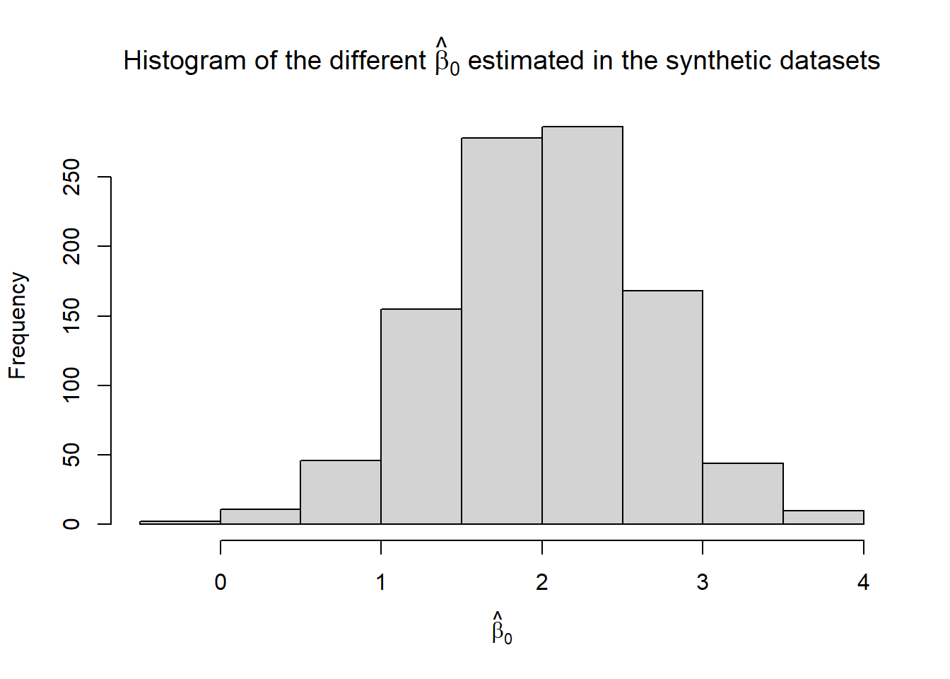
hist(b1.hat, xlab = TeX("$\\hat{\\beta}_1$"),
     main = TeX("Histogram of the different $\\hat{\\beta}_1$ estimated in the synthetic datasets"))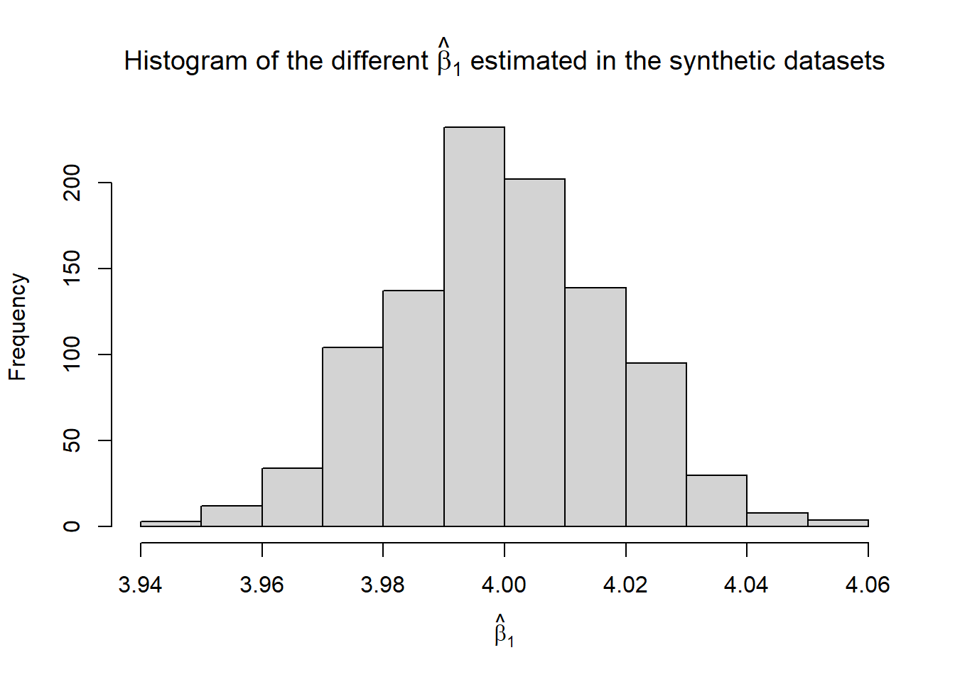
paste0("In the 1000 simulated scenarios, the confidence interval included the true beta_0 ",
       100*mean(b0.hat.calib), "% of the times.", sep = "")
## [1] "In the 1000 simulated scenarios, the confidence interval included the true beta_0 95.9% of the times."paste0("In the 1000 simulated scenarios, the confidence interval included the true beta_1 ",
100*mean(b1.hat.calib), "% of the times.", sep = "")## [1] "In the 1000 simulated scenarios, the confidence interval included the true beta_1 95.9% of the times."21.3 Power analysis demonstration
We’ll simulate the design of an experiment. Let’s assume the following:
3 \(\times\) 2 factorial treatment structure, with temperature at 250, 400, and 500 F, and 2 muffin recipes.
Treatment means: \(\mu_{11}=2\), \(\mu_{21}=2.4\), \(\mu_{31}=2.6\), \(\mu_{12}=2.4\), \(\mu_{22}=2.8\), \(\mu_{32}=3\).
Which means: \(\mu_{1\cdot} - \mu_{2\cdot} = -0.4\), \(\mu_{1\cdot} - \mu_{2\cdot} = -0.4\).
Consider these competing designs:
- CRD
- split-plot design
- split-plot design with subsampling
All examples below generate 100 designs with the means described above, the designs with 2 or 3 repetitions, and the corresponding variances for each design (e.g., \(\sigma^2_\varepsilon\), \(\sigma^2_{whole plot}\), etc.).
21.3.1 CRD - 2 reps
df_crd <- expand.grid(oven_temp = factor(c(250, 400, 500)),
                      recipe = c("B", "C"),
                      rep = 1:2)
df_crd <- df_crd %>%
  mutate(mu = case_when(oven_temp == "250" & recipe == "B" ~ 2,
                        oven_temp == "400" & recipe == "B" ~ 2.4,
                        oven_temp == "500" & recipe == "B" ~ 2.6,
                        oven_temp == "250" & recipe == "C" ~ 2.4,
                        oven_temp == "400" & recipe == "C" ~ 2.8,
                        oven_temp == "500" & recipe == "C" ~ 3))

sigma_epsilon <- 0.26


n_sims <- 100
p_mu.1_mu.2 <- numeric(n_sims)
p_mu1._mu2. <- numeric(n_sims)

n <- nrow(df_crd)set.seed(42)
for (i in 1:n_sims){
df_temp <- df_crd %>% mutate(y = mu + rnorm(n, 0, sigma_epsilon))
m <- lm(y ~ oven_temp * recipe, data = df_temp)
p_mu.1_mu.2[i] <- as.data.frame(emmeans(m, ~recipe, contr = list(c(1, -1)))$contrasts)$p.value
p_mu1._mu2.[i] <- as.data.frame(emmeans(m, ~oven_temp, contr = list(c(1, -1, 0)))$contrasts)$p.value
}hist(p_mu.1_mu.2,
xlim = c(0, 1),
xlab = TeX("$\\hat{\\mu}_{\\cdot 1} - \\hat{\\mu}_{\\cdot 2}$"),
main = TeX("p-value for $\\hat{\\mu}_{\\cdot 1} - \\hat{\\mu}_{\\cdot 2}$ under a CRD with 2 reps"))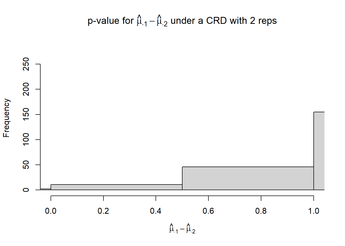
hist(p_mu1._mu2.,
     xlim = c(0, 1),
     xlab = TeX("$\\hat{\\mu}_{1 \\cdot} - \\hat{\\mu}_{2 \\cdot}$"),
     main = TeX("p-value for $\\hat{\\mu}_{1 \\cdot} - \\hat{\\mu}_{2 \\cdot}$ under a CRD with 2 reps"))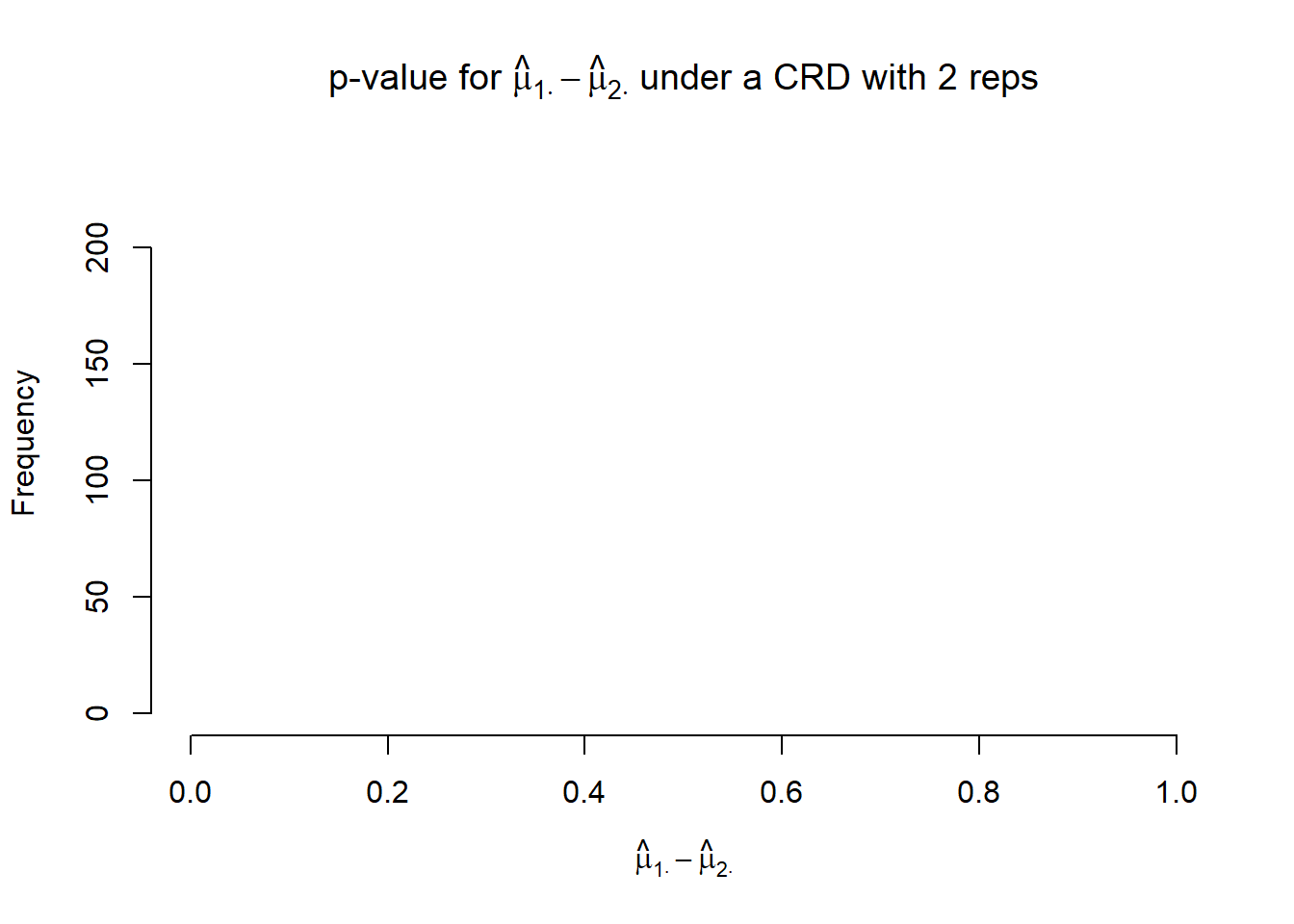
## [1] 0.002## [1] 021.3.2 CRD - 3 reps
df_crd <- expand.grid(oven_temp = factor(c(250, 400, 500)),
                      recipe = c("B", "C"),
                      rep = 1:3)
df_crd <- df_crd %>%
  mutate(mu = case_when(oven_temp == "250" & recipe == "B" ~ 2,
                        oven_temp == "400" & recipe == "B" ~ 2.4,
                        oven_temp == "500" & recipe == "B" ~ 2.6,
                        oven_temp == "250" & recipe == "C" ~ 2.4,
                        oven_temp == "400" & recipe == "C" ~ 2.8,
                        oven_temp == "500" & recipe == "C" ~ 3))

sigma_epsilon <- 0.26


p_mu.1_mu.2 <- numeric(n_sims)
p_mu1._mu2. <- numeric(n_sims)

n <- nrow(df_crd)

set.seed(42)
for (i in 1:n_sims){
df_temp <- df_crd %>% mutate(y = mu + rnorm(n, 0, sigma_epsilon))
m <- lm(y ~ oven_temp * recipe, data = df_temp)
p_mu.1_mu.2[i] <- as.data.frame(emmeans(m, ~recipe, contr = list(c(1, -1)))$contrasts)$p.value
p_mu1._mu2.[i] <- as.data.frame(emmeans(m, ~oven_temp, contr = list(c(1, -1, 0)))$contrasts)$p.value
}hist(p_mu.1_mu.2,
xlim = c(0, 1),
xlab = TeX("$\\hat{\\mu}_{\\cdot 1} - \\hat{\\mu}_{\\cdot 2}$"),
main = TeX("p-value for $\\hat{\\mu}_{\\cdot 1} - \\hat{\\mu}_{\\cdot 2}$ under a CRD with 3 reps"))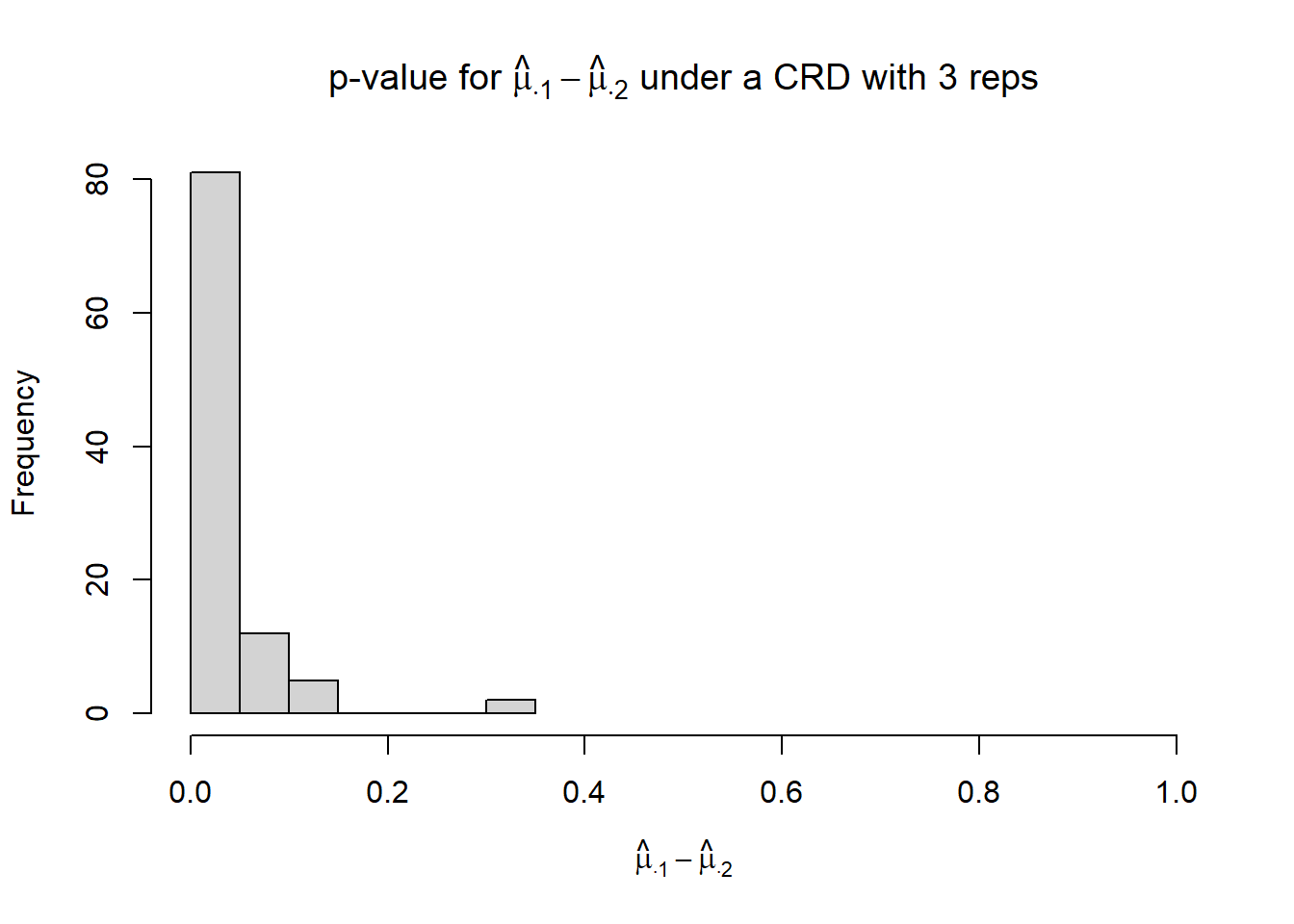
hist(p_mu1._mu2.,
     xlim = c(0, 1),
     xlab = TeX("$\\hat{\\mu}_{1 \\cdot} - \\hat{\\mu}_{2 \\cdot}$"),
     main = TeX("p-value for $\\hat{\\mu}_{1 \\cdot} - \\hat{\\mu}_{2 \\cdot}$ under a CRD with 3 reps"))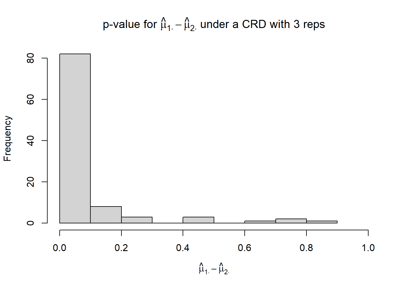
## [1] 0.81## [1] 0.7121.3.3 Split-plot - 2 reps
df_splitplot <-
  expand.grid(oven_temp = factor(c(250, 400, 500)),
              recipe = c("B", "C"),
              rep = 1:2) %>%
  mutate(wp_id = as.numeric(as.factor(paste(oven_temp, rep))))

df_splitplot <- df_splitplot %>%
  mutate(mu = case_when(oven_temp == "250" & recipe == "B" ~ 2,
                        oven_temp == "400" & recipe == "B" ~ 2.4,
                        oven_temp == "500" & recipe == "B" ~ 2.6,
                        oven_temp == "250" & recipe == "C" ~ 2.4,
                        oven_temp == "400" & recipe == "C" ~ 2.8,
                        oven_temp == "500" & recipe == "C" ~ 3))

sigma_epsilon <- 0.26
sigma_oven <- .12
n <- nrow(df_splitplot)
n_wp <- n_distinct(df_splitplot$oven_temp) * n_distinct(df_splitplot$rep)

p_mu.1_mu.2 <- numeric(n_sims)
p_mu1._mu2. <- numeric(n_sims)set.seed(42)
for (i in 1:n_sims){
oven_re <- rnorm(n_wp, 0, sigma_oven)
df_temp <- df_splitplot %>% mutate(y = mu + oven_re[wp_id] + rnorm(n, 0, sigma_epsilon) )
m <- lmer(y ~ oven_temp * recipe + (1|oven_temp:rep), data = df_temp)
p_mu.1_mu.2[i] <- as.data.frame(emmeans(m, ~recipe, contr = list(c(1, -1)))$contrasts)$p.value
p_mu1._mu2.[i] <- as.data.frame(emmeans(m, ~oven_temp, contr = list(c(1, -1, 0)))$contrasts)$p.value
}hist(p_mu.1_mu.2,
xlim = c(0, 1),
xlab = TeX("$\\hat{\\mu}_{\\cdot 1} - \\hat{\\mu}_{\\cdot 2}$"),
main = TeX("p-value for $\\hat{\\mu}_{\\cdot 1} - \\hat{\\mu}_{\\cdot 2}$ under a split-plot design with 2 reps"))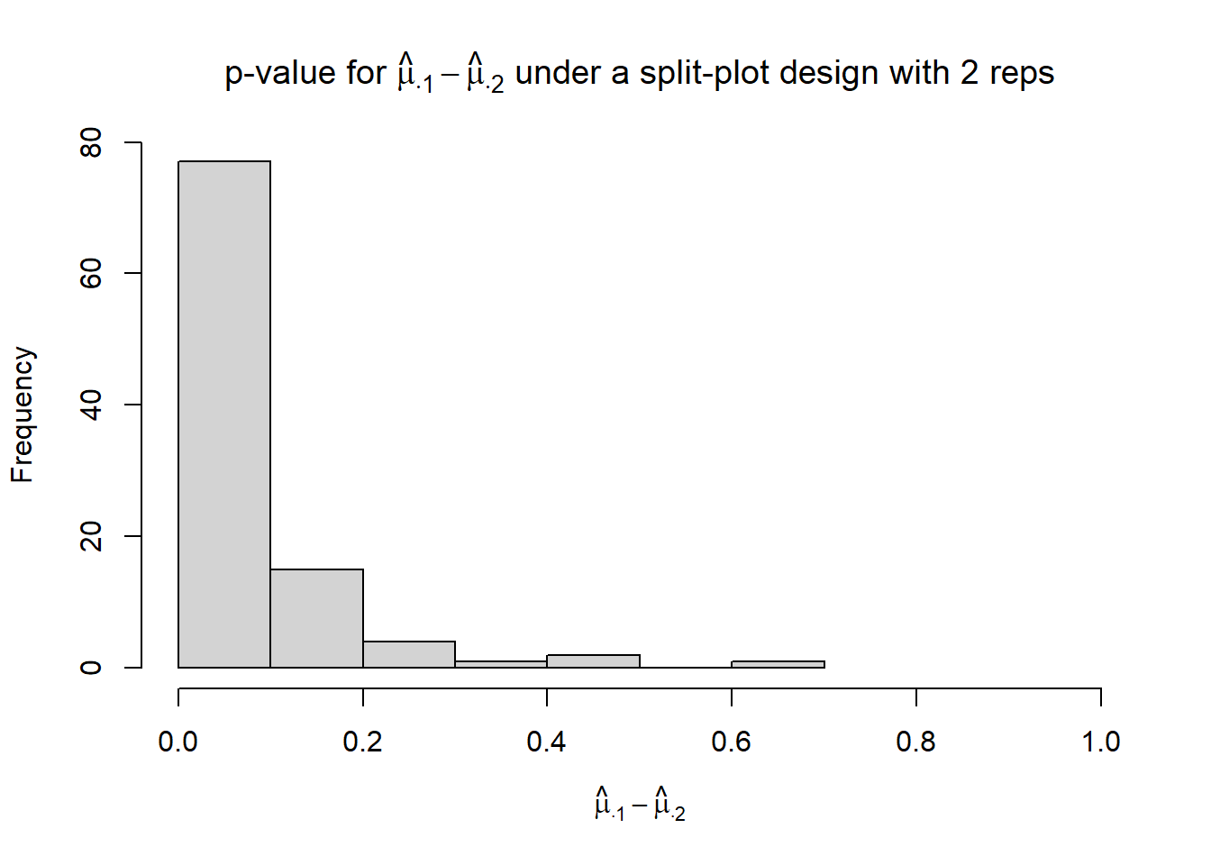
hist(p_mu1._mu2.,
     xlim = c(0, 1),
     xlab = TeX("$\\hat{\\mu}_{1 \\cdot} - \\hat{\\mu}_{2 \\cdot}$"),
     main = TeX("p-value for $\\hat{\\mu}_{1 \\cdot} - \\hat{\\mu}_{2 \\cdot}$ under a split-plot design with 2 reps"))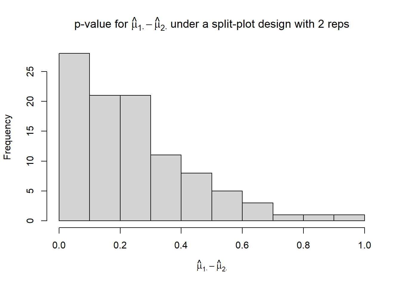
## [1] 0.56## [1] 0.1121.3.4 Split-plot - 3 reps
df_splitplot <-
  expand.grid(oven_temp = factor(c(250, 400, 500)),
              recipe = c("B", "C"),
              rep = 1:3) %>%
  mutate(wp_id = as.numeric(as.factor(paste(oven_temp, rep))))

df_splitplot <- df_splitplot %>%
  mutate(mu = case_when(oven_temp == "250" & recipe == "B" ~ 2,
                        oven_temp == "400" & recipe == "B" ~ 2.4,
                        oven_temp == "500" & recipe == "B" ~ 2.6,
                        oven_temp == "250" & recipe == "C" ~ 2.4,
                        oven_temp == "400" & recipe == "C" ~ 2.8,
                        oven_temp == "500" & recipe == "C" ~ 3))

sigma_epsilon <- 0.26
sigma_oven <- .12
n <- nrow(df_splitplot)
n_wp <- n_distinct(df_splitplot$oven_temp) * n_distinct(df_splitplot$rep)

p_mu.1_mu.2 <- numeric(n_sims)
p_mu1._mu2. <- numeric(n_sims)set.seed(42)
for (i in 1:n_sims){
oven_re <- rnorm(n_wp, 0, sigma_oven)
df_temp <- df_splitplot %>% mutate(y = mu + oven_re[wp_id] + rnorm(n, 0, sigma_epsilon) )
m <- lmer(y ~ oven_temp * recipe + (1|oven_temp:rep), data = df_temp)
p_mu.1_mu.2[i] <- as.data.frame(emmeans(m, ~recipe, contr = list(c(1, -1)))$contrasts)$p.value
p_mu1._mu2.[i] <- as.data.frame(emmeans(m, ~oven_temp, contr = list(c(1, -1, 0)))$contrasts)$p.value
}hist(p_mu.1_mu.2,
xlim = c(0, 1),
xlab = TeX("$\\hat{\\mu}_{\\cdot 1} - \\hat{\\mu}_{\\cdot 2}$"),
main = TeX("p-value for $\\hat{\\mu}_{\\cdot 1} - \\hat{\\mu}_{\\cdot 2}$ under a split-plot design with 3 reps"))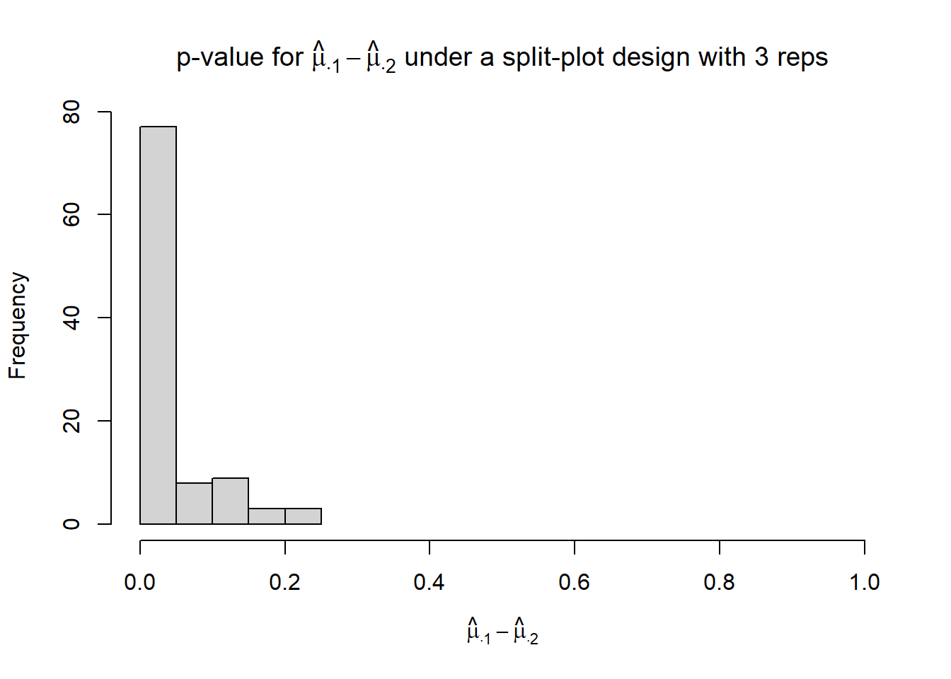
hist(p_mu1._mu2.,  xlab = TeX("$\\hat{\\mu}_{1 \\cdot} - \\hat{\\mu}_{2 \\cdot}$"),
     main = TeX("p-value for $\\hat{\\mu}_{1 \\cdot} - \\hat{\\mu}_{2 \\cdot}$ under a split-plot design with 3 reps"))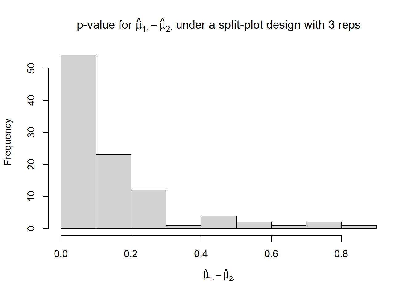
## [1] 0.77## [1] 0.3821.3.5 Split-plot - 2 reps + subsampling
df_splitplot_subsample <-
  expand.grid(oven_temp = factor(c(250, 400, 500)),
              recipe = c("B", "C"),
              rep = 1:2,
              subsample = 1:3) %>%
  mutate(wp_id = as.numeric(as.factor(paste(rep, oven_temp))),
         muffin_id = as.numeric(as.factor(paste(rep, oven_temp, recipe))))

df_splitplot_subsample <- df_splitplot_subsample %>%
  mutate(mu = case_when(oven_temp == "250" & recipe == "B" ~ 2,
                        oven_temp == "400" & recipe == "B" ~ 2.4,
                        oven_temp == "500" & recipe == "B" ~ 2.6,
                        oven_temp == "250" & recipe == "C" ~ 2.4,
                        oven_temp == "400" & recipe == "C" ~ 2.8,
                        oven_temp == "500" & recipe == "C" ~ 3))

sigma_epsilon <- 0.26
sigma_oven <- .12
sigma_muffins <- .1

n <- nrow(df_splitplot)
n_wp <- n_distinct(df_splitplot$oven_temp) * n_distinct(df_splitplot$rep)
n_sp <- n_distinct(df_splitplot$oven_temp) * n_distinct(df_splitplot$rep) * n_distinct(df_splitplot$recipe)

p_mu.1_mu.2 <- numeric(n_sims)
p_mu1._mu2. <- numeric(n_sims)set.seed(42)
for (i in 1:n_sims){
oven_re <- rnorm(n_wp, 0, sigma_oven)
muffins_re <- rnorm(n_sp, 0, sigma_muffins)
df_temp <- df_splitplot_subsample %>%
mutate(y = mu + oven_re[wp_id] + muffins_re[muffin_id] +
rnorm(n, 0, sigma_epsilon) )
m <- lmer(y ~ oven_temp * recipe + (1|oven_temp:rep/recipe), data = df_temp)
p_mu.1_mu.2[i] <- as.data.frame(emmeans(m, ~recipe, contr = list(c(1, -1)))$contrasts)$p.value
p_mu1._mu2.[i] <- as.data.frame(emmeans(m, ~oven_temp, contr = list(c(1, -1, 0)))$contrasts)$p.value
}hist(p_mu.1_mu.2,
xlim = c(0, 1),
xlab = TeX("$\\hat{\\mu}_{\\cdot 1} - \\hat{\\mu}_{\\cdot 2}$"),
main = TeX("p-value for $\\hat{\\mu}_{\\cdot 1} - \\hat{\\mu}_{\\cdot 2}$ under a split-plot design with 2 reps and subsampling"))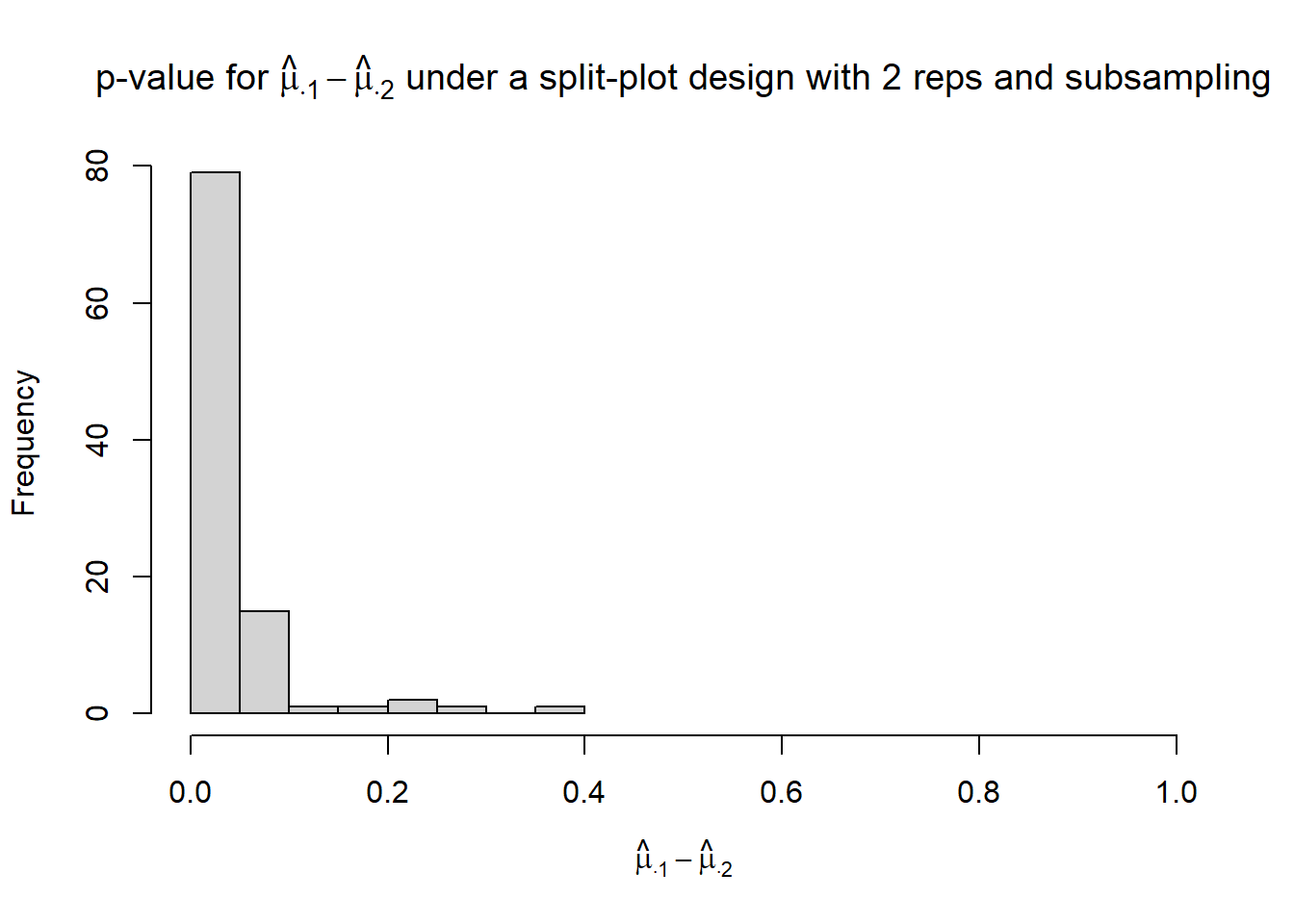
hist(p_mu1._mu2.,
     xlim = c(0, 1),
     xlab = TeX("$\\hat{\\mu}_{1 \\cdot} - \\hat{\\mu}_{2 \\cdot}$"),
     main = TeX("p-value for $\\hat{\\mu}_{1 \\cdot} - \\hat{\\mu}_{2 \\cdot}$ under a split-plot design with 2 reps and subsampling"))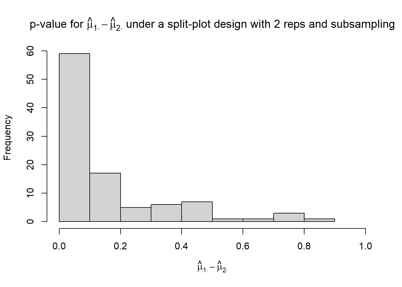
## [1] 0.79## [1] 0.4121.3.6 Split-plot - 3 reps + subsampling
df_splitplot_subsample <-
  expand.grid(oven_temp = factor(c(250, 400, 500)),
              recipe = c("B", "C"),
              rep = 1:4,
              subsample = 1:3) %>%
  mutate(wp_id = as.numeric(as.factor(paste(rep, oven_temp))),
         muffin_id = as.numeric(as.factor(paste(rep, oven_temp, recipe))))

df_splitplot_subsample <- df_splitplot_subsample %>%
  mutate(mu = case_when(oven_temp == "250" & recipe == "B" ~ 2,
                        oven_temp == "400" & recipe == "B" ~ 2.4,
                        oven_temp == "500" & recipe == "B" ~ 2.6,
                        oven_temp == "250" & recipe == "C" ~ 2.4,
                        oven_temp == "400" & recipe == "C" ~ 2.8,
                        oven_temp == "500" & recipe == "C" ~ 3))

sigma_epsilon <- 0.26
sigma_oven <- .12
sigma_muffins <- .1

n <- nrow(df_splitplot)
n_wp <- n_distinct(df_splitplot$oven_temp) * n_distinct(df_splitplot$rep)
n_sp <- n_distinct(df_splitplot$oven_temp) * n_distinct(df_splitplot$rep) * n_distinct(df_splitplot$recipe)

p_mu.1_mu.2 <- numeric(n_sims)
p_mu1._mu2. <- numeric(n_sims)set.seed(3)
for (i in 1:n_sims){
oven_re <- rnorm(n_wp, 0, sigma_oven)
muffins_re <- rnorm(n_sp, 0, sigma_muffins)
df_temp <- df_splitplot_subsample %>%
mutate(y = mu + oven_re[wp_id] + muffins_re[muffin_id] +
rnorm(n, 0, sigma_epsilon) )
m <- lmer(y ~ oven_temp * recipe + (1|oven_temp:rep/recipe), data = df_temp)
p_mu.1_mu.2[i] <- as.data.frame(emmeans(m, ~recipe, contr = list(c(1, -1)))$contrasts)$p.value
p_mu1._mu2.[i] <- as.data.frame(emmeans(m, ~oven_temp, contr = list(c(1, -1, 0)))$contrasts)$p.value
}hist(p_mu.1_mu.2,
xlim = c(0, 1),
xlab = TeX("$\\hat{\\mu}_{\\cdot 1} - \\hat{\\mu}_{\\cdot 2}$"),
main = TeX("p-value for $\\hat{\\mu}_{\\cdot 1} - \\hat{\\mu}_{\\cdot 2}$ under a split-plot design with 3 reps and subsampling"))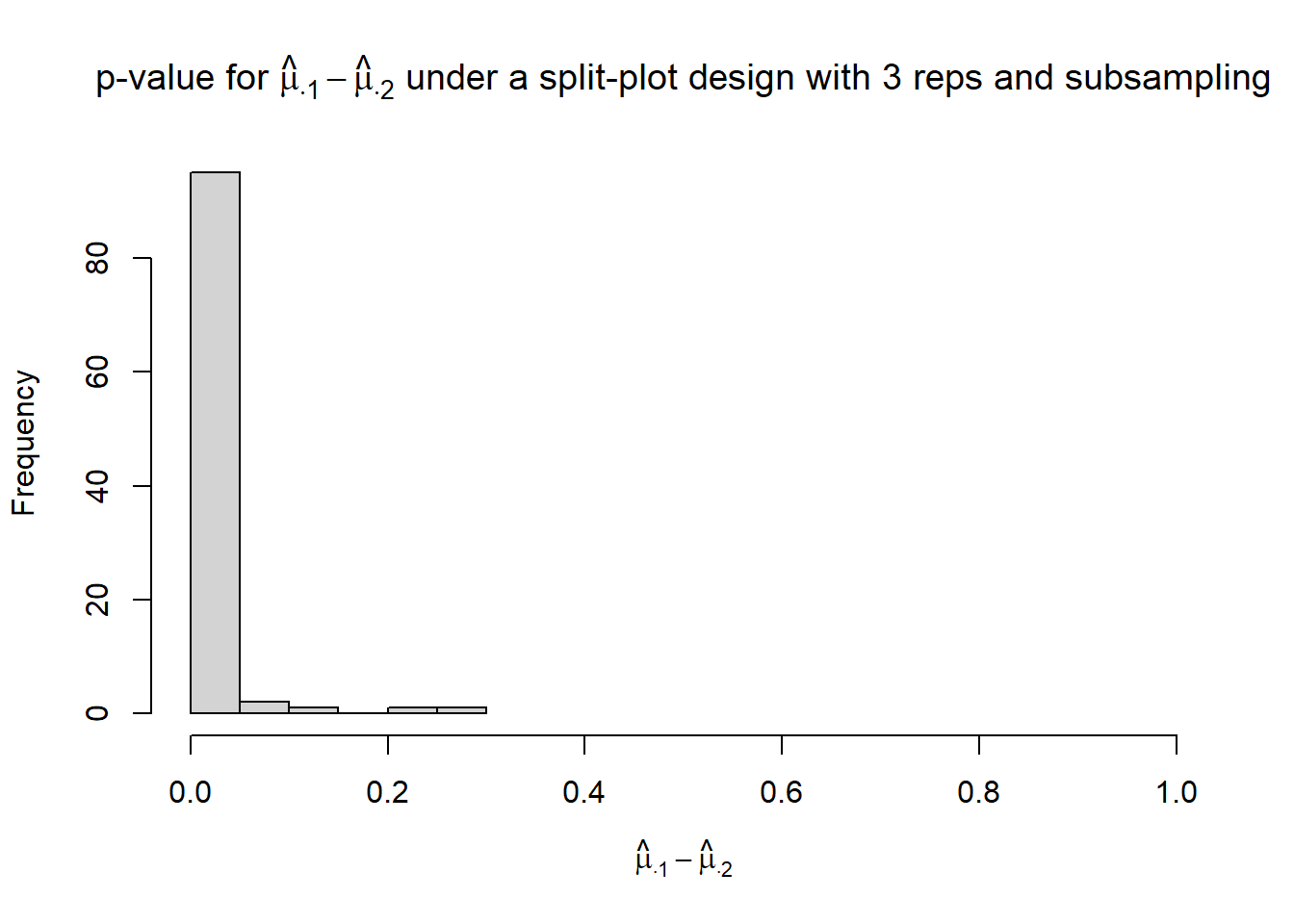
hist(p_mu1._mu2.,
     xlim = c(0, 1),
     xlab = TeX("$\\hat{\\mu}_{1 \\cdot} - \\hat{\\mu}_{2 \\cdot}$"),
     main = TeX("p-value for $\\hat{\\mu}_{1 \\cdot} - \\hat{\\mu}_{2 \\cdot}$ under a split-plot design with 3 reps and subsampling"))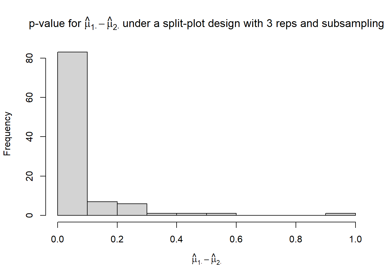
## [1] 0.95## [1] 0.71