Day 27 Crossover Designs I
July 21st, 2025
27.2 Crossover designs
- Apply treatments to the same experimental unit sequentially, to eliminate between-experimental unit variation when comparing treatments
- \(t\) treatments are compared where each treatment is observed on each of the experimental units (i.e., the treatments are applied in a specified sequence to the experimental units).
- Mostly applied in animal studies.
- In non-crossover designs: \(y_{ik} = \mu + T_i+ \varepsilon_{ik}\), where \(y_{ijk}\) is the observation for the \(i\)th treatment and the \(k\)th individual, \(T_i\) is the effect of the \(i\)th treatment, and \(\varepsilon_{ij}\) is the residual that includes the variability between individuals (i.e., experimental units).
- In crossover designs, \(y_{ijkl} = \mu + T_i + P_j + S_k + u_l + \varepsilon_{ijkl}\),where \(y_{ijk}\) is the observation for the \(i\)th treatment, \(j\)th period for the \(l\)th individual that received the treatments in the \(k\)th sequence, \(T_i\) is the effect of the \(i\)th treatment, \(P_j\) is the effect of the \(j\)th period, \(S_k\) is the effect of the \(k\)th sequence, \(u_l\) is the (random) effect of the \(l\)th individual under the \(k\)th sequence, and \(\varepsilon_{ijkl}\) is the residual.
- Potential problems: carryover or residual effects.
- More in Chapter 29 in the Messy Data book.
Pros:
- Fewer EUs (probably living beings) required
- Power (?)
- Between-EU variability is accounted for in the model
Cons:
- Carryover (residual) effects
- Power (!?)
- Longer duration of the experiment
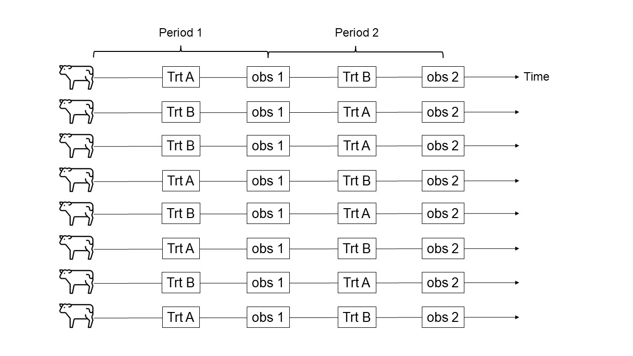
Figure 27.1: Schematic representation of a crossover design
Example study the effect of \(k\) treatments on response \(y\):
This study was published in Grizzle (1965). This study studied the effect of 2 drugs (A and B) on humans. First, 28 persons were randomly assigned one of two drugs, and the trait of study was measured at the end of the treatment duration. Then, all persons were given the other drug they hadn’t taken yet.
df <- read.csv("https://raw.githubusercontent.com/stat720/summer2025/refs/heads/main/data/grizzle_messydata.csv")
df$Period <- as.factor(df$Period)
df$Person <- as.factor(df$Person)

m <- lmer(Y ~ Seq + Trt + Period + (1|Seq:Person) , data = df)

car::Anova(m, type = 3, test.statistic = "F")
## Analysis of Deviance Table (Type III Wald F tests with Kenward-Roger df)
##
## Response: Y
## F Df Df.res Pr(>F)
## (Intercept) 0.0017 1 12 0.96783
## Seq 4.0726 1 12 0.06651 .
## Trt 3.1729 1 12 0.10018
## Period 5.5594 1 12 0.03619 *
## ---
## Signif. codes: 0 '***' 0.001 '**' 0.01 '*' 0.05 '.' 0.1 ' ' 1## [1] 14## contrast estimate SE df t.ratio p.value
## c(1, -1) 0.721 0.405 12 1.781 0.1002
##
## Results are averaged over the levels of: Seq, Period
## Degrees-of-freedom method: kenward-roger