Day 29 That’s all folks!
July 23rd, 2025
29.2 Principles for conducting valid and efficient experiments

Figure 29.1: ‘Principles for conducting valid and efficient experiments’. From Box, Hunter and Hunter (2005).
29.3 Modeling data generated by designed experiments
- The most common model that is the default in most software: \(y_{ij} = \mu + T_i + \varepsilon_{ij} , \ \varepsilon_{ij}\sim N(0, \sigma^2)\).
- Independence
- Constant variance
- Normal distribution
- Designed experiments sometimes handle EUs in groups, leaving us with groups of data that have something in common rather than being independent.
- Different patterns of “similar groups” lead to us calling them different designs.
- Blocked designs - randomized complete block designs, incomplete block designs
- Multilevel designs: split-plot designs, multi-location designs, subsampling, etc.
- Crossover designs
- Repeated measures (Time is one of the treatment factors)
- Comment: repeated measures in SAS and in R
- What is what? Sketch it!
- Inter-block recovery of information for incomplete block designs
- One model versus dividing the data
- The importance of writing the statistical model!
29.3.1 From ANOVA table to statistical model
|
|
|
The statistical model corresponding to this ANOVA table was \[y_{ijk} = \mu + \delta_k + T_i + w_{i(k)} + R_j + TR_{ij} + \varepsilon_{ijk},\] where:
\(y_{ijk}\) is the observation of the height of a muffin baked on day \(k\) under the \(i\)th temperature, prepared with the \(i\)th recipe,
\(\mu\) is the overall mean,
\(\delta_k\) is the effect of day \(k\),
\(T_i\) is the effect of the \(i\)th temperature,
\(w_{i(k)}\) is the effect of over at the \(i\)th temperature on day \(k\),
\(R_j\) is the effect of the \(j\)th recipe,
\(TR_{ij}\) is the interaction between the \(i\)th temperature and \(j\)th recipe,
\(\varepsilon_{ijk}\) is the residual for the height of a muffin baked on day \(k\) under the \(i\)th temperature, prepared with the \(i\)th recipe.
Effects model versus Means model
29.3.2 What happens if we drop blocks, split-plots, etc?
What if the elements of the design (blocks, whole plots) are not significant?
- Interpreting a small variance component (e.g., \(\sigma^2_b\) ) vs. a non-significant fixed effect (i.e., \(p_B >0.05\) )
- The Difference Between “Significant” and “Not Significant” is not Itself Statistically Significant - Gelman and Stern (2012)
- Currently, the general advice is to include the randomization structure to avoid type I error deflation – see “Analyze as randomized – Why dropping block effects in designed experiments is a bad idea (Frey et al., 2024)”
- Review on split-plot designs, EU sizes, and subsampling/pseudoreplication.
29.3.3 Differences modeling multi-location designed experiments
- Random effects versus fixed effects assumptions
- Remember that you are designing a model that describes how the data were generated, not using the model that will fit the results you hope to get.
- See Gelman (2005) - page 20.
Example: sites that are somewhat different
- An argument against “On the other hand, modeling location as a fixed effect restricts inference to those specific locations only. Therefore, if the goal is to make inferences across a broader region or range of conditions, treating location as a random effect is the preferred approach.”
## 'data.frame':    72 obs. of  5 variables:
##  $ gen  : Factor w/ 12 levels "Cap","Dur","Fun",..: 1 1 1 1 1 1 7 7 7 7 ...
##  $ loc  : Factor w/ 7 levels "Beg","Box","Cra",..: 3 3 1 1 5 5 3 3 1 1 ...
##  $ nitro: Factor w/ 2 levels "H","L": 2 1 2 1 2 1 2 1 2 1 ...
##  $ yield: int  321 411 317 429 566 625 285 436 328 450 ...
##  $ type : Factor w/ 2 levels "conv","semi": 1 1 1 1 1 1 1 1 1 1 ...
m_fixed <- lm(yield ~ nitro*type + loc, data = df_env2)
m_random <- lmer(yield ~ nitro*type + (1|loc), data = df_env2)The marginal means look the same…
##  nitro type emmean   SE df lower.CL upper.CL
##  H     conv    527 17.9 66      492      563
##  L     conv    448 17.9 66      412      484
##  H     semi    561 15.1 66      531      591
##  L     semi    473 15.1 66      443      503
##
## Results are averaged over the levels of: loc
## Confidence level used: 0.95## nitro type emmean SE df lower.CL upper.CL
## H conv 527 111 2.09 69.82 985
## L conv 448 111 2.09 -9.58 905
## H semi 561 110 2.05 98.57 1023
## L semi 473 110 2.05 10.62 935
##
## Degrees-of-freedom method: kenward-roger
## Confidence level used: 0.95… but the CI is sooooo much wider for the mean of the mixed model!
##   nitro type   emmean       SE df lower.CL upper.CL CI_width
## 1     H conv 527.3333 17.87558 66 491.6436 563.0231 71.37948
## 2     L conv 447.9333 17.87558 66 412.2436 483.6231 71.37948
## 3     H semi 560.6667 15.10762 66 530.5033 590.8300 60.32667
## 4 L semi 472.7143 15.10762 66 442.5509 502.8776 60.32667## nitro type emmean SE df lower.CL upper.CL CI_width
## 1 H conv 527.3333 110.5595 2.085395 69.822265 984.8444 915.0221
## 2 L conv 447.9333 110.5595 2.085395 -9.577735 905.4444 915.0221
## 3 H semi 560.6667 110.1458 2.054377 98.567596 1022.7657 924.1981
## 4 L semi 472.7143 110.1458 2.054377 10.615216 934.8134 924.1981Now let’s take a look at the residual quantiles:
simres1 <- DHARMa::simulateResiduals(m_fixed, plot = F)
DHARMa::plotQQunif(simres1, main = "QQ plot residuals - fixed model")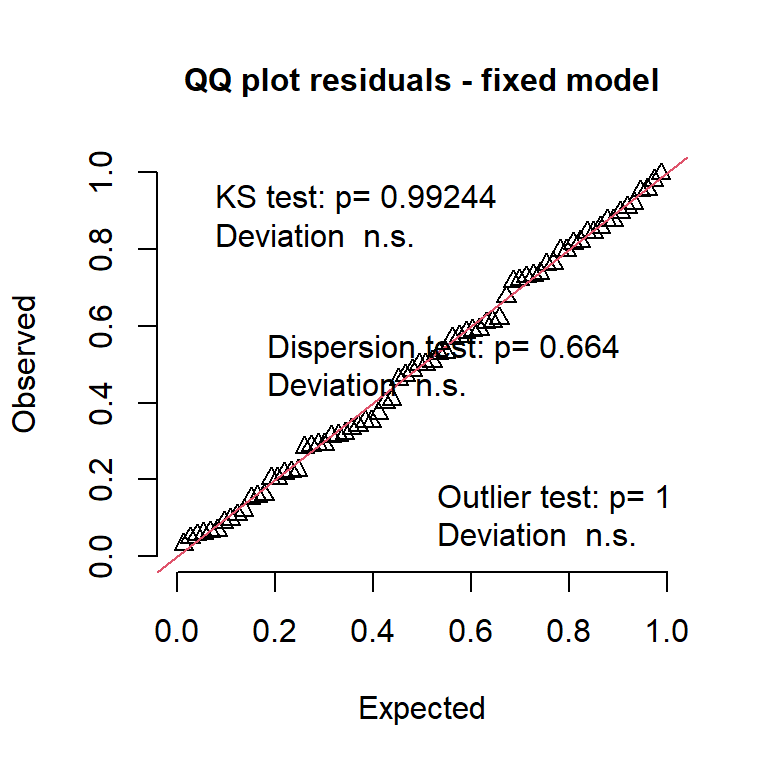
simres2 <- DHARMa::simulateResiduals(m_random, use.u = F)
DHARMa::plotQQunif(simres2, main = "QQ plot residuals - mixed model w/o RE")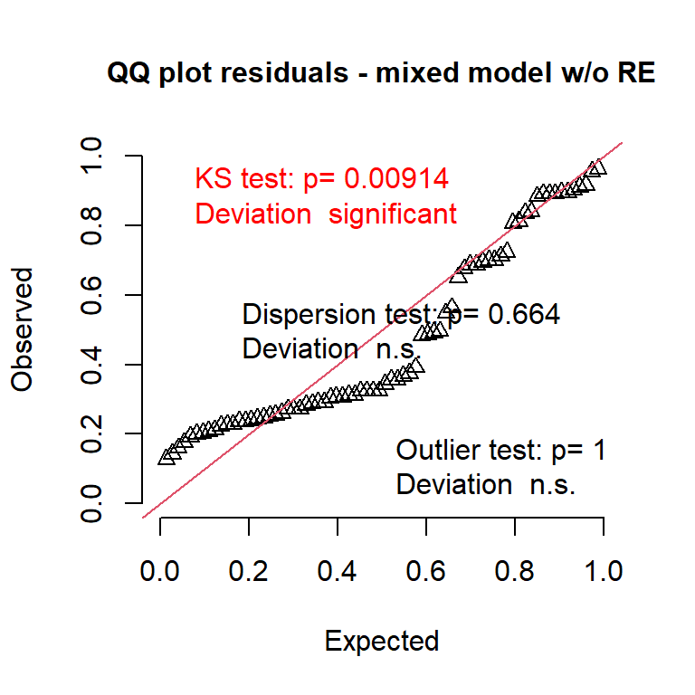
simres3 <- DHARMa::simulateResiduals(m_random, use.u = T)
DHARMa::plotQQunif(simres3, main = "QQ plot residuals - mixed model")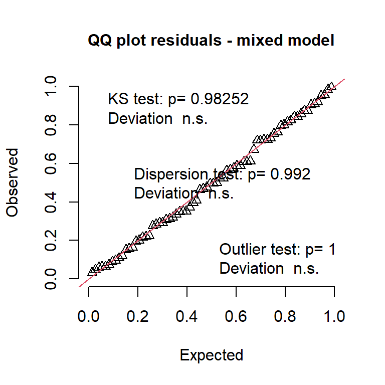
What is happening??
Shrinkage:
Take a look at \(\hat{L}\) (fixed location effect):
## [1] -90.16667 -127.58333 217.75000And then take a look at \(\hat{l}\) (random location effect):
## [1] -89.66523 -126.87382 216.53905Figure 29.2: ‘Principles for conducting valid and efficient experiments’. From Box, Hunter and Hunter (2005).
29.4 Learn more about designing and analyzing experiments
- Mixed models workshops in the Fall
- Messy Data (STAT 870) in the Fall
- Categorical Data Analysis (STAT 717) in the Spring
- Other resources:
- Stroup et al. 2024
- Andrew Gelman’s (& friends) blog