Day 24 Split plot designs

July 15th, 2025

24.1 Announcements

• HW 4 due Friday

24.2 Split plot designs

• Split-plot designs are multi-level designed experiments.
• Randomization happens in different domains.

Let’s look at two alternatives for randomizing the whole-plot factor levels, in a CRD and in a blocked scenario:

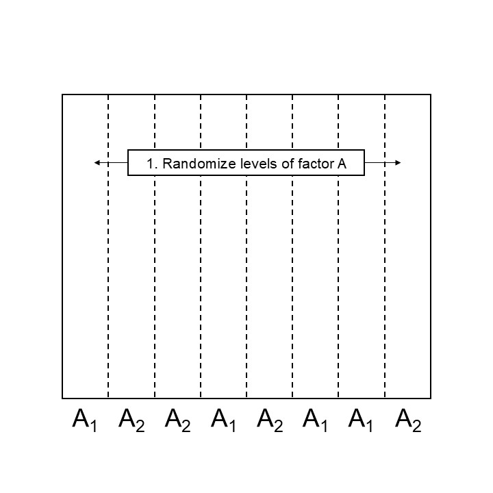
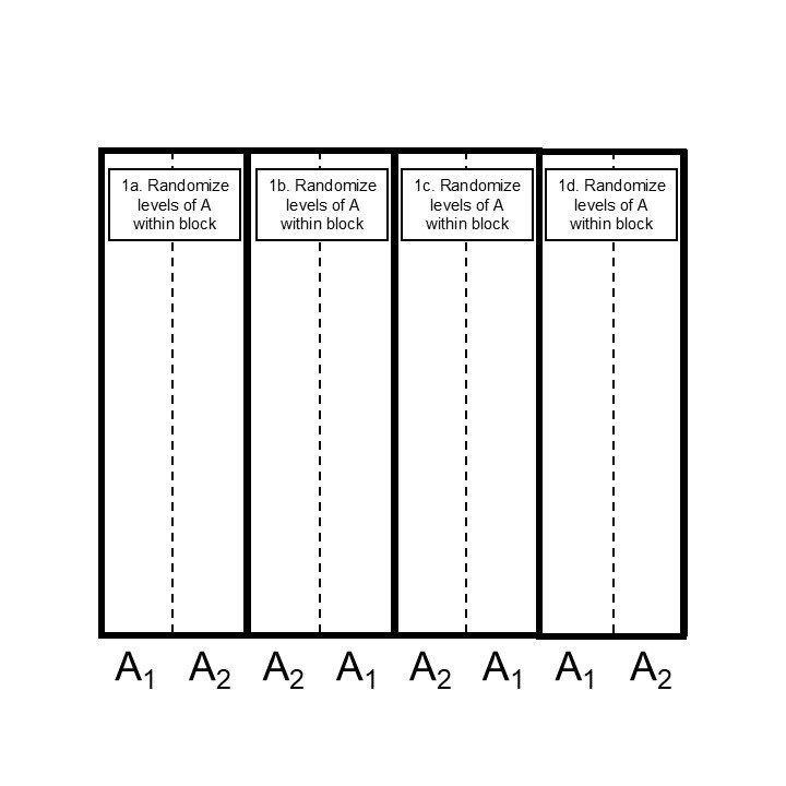
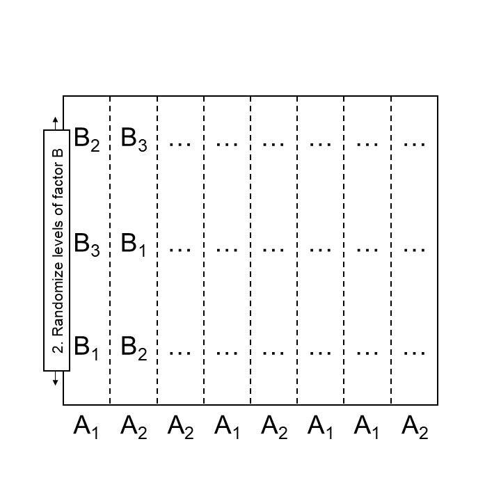
Figure 24.1: Step 2 designing a split plot design

Remember:

• Blocks are groups of approximately similar experimental units.
• Data generated by blocked designs may be analyzed as \(y_{ij} = \mu +\tau_i + b_j + \varepsilon_{ij}\), where \(y_{ij}\) is the observed response for the \(i\)th treatment in the \(j\)th block, \(\tau_i\) is the effect of the \(i\)th treatment, \(b_j\) is the effect of the \(j\)th block, \(\varepsilon_{ij}\) is the residual of the \(i\)th treatment in the \(j\)th block.
• Data generated by split-plot designs may be analyzed as \(y_{ijk} = \mu + T_i +A_j +(TA)_{ij} + b_k + w_{i(k)} + \varepsilon_{ij}\), where \(y_{ij}\) is the observed response for the \(i\)th level of factor T, the \(j\)th level of factor A, in the \(k\)th block, \(T_i\) is the effect of the \(i\)th level of treatment T, \(A_j\) is the effect of the \(j\)th level of treatment A, \(b_k\) is the effect of block \(k\) and may be random or fixed, \(w_i(k)\) is the effect of the whole plot corresponding to the \(i\)th treatment T in block \(k\), and \(\varepsilon_{ijk}\) is the residual of the \(i\)th level of factor T, the \(j\)th level of factor A, in the \(k\)th block.
• Typically assume \(w_{i(k)} \sim N(0, \sigma^2_w)\).
• \(b_k\) may still be fixed or random.
• Variance components should be \(> 0\).

24.2.1 Applied case: split-plot design

Grain yield was measured at for a split-plot experiment of barley with fungicide treatments. Within each block, fungicides were randomized and then, barley varieties were randomly applied to smaller plots.

library(tidyverse)
library(agridat)
library(lme4)
library(emmeans)

df_splitplot <- agridat::durban.splitplot

m_splitplot <- lmer(yield ~ fung * gen + (1|block/fung), 
                    data = df_splitplot)

VarCorr(m_splitplot)

##  Groups     Name        Std.Dev.
##  fung:block (Intercept) 0.11737 
##  block      (Intercept) 0.16972 
##  Residual               0.28119

24.2.1.1 Standard errors

sigma2_e <- sigma(m_splitplot)^2
sigma2_wp <- as.data.frame(VarCorr(m_splitplot))[1,]$vcov
sigma2_b <- as.data.frame(VarCorr(m_splitplot))[2,]$vcov
levels_wp <- n_distinct(df_splitplot$fung)
levels_sp <- n_distinct(df_splitplot$gen)
reps <- n_distinct(df_splitplot$block)

Mean differences for factor at the whole plot

sqrt( 2*(sigma2_e + levels_sp*sigma2_wp) / (levels_sp*reps))

## [1] 0.086331

emmeans(m_splitplot, ~fung, contr = list(c(1, -1)))$contr

## NOTE: Results may be misleading due to involvement in interactions

##  contrast estimate     SE df t.ratio p.value
##  c(1, -1)    0.548 0.0863  3   6.346  0.0079
## 
## Results are averaged over the levels of: gen 
## Degrees-of-freedom method: kenward-roger

Mean differences for factor at the sub plot

sqrt( 2*(sigma2_e ) / (levels_wp*reps))

## [1] 0.1405927

emmeans(m_splitplot, ~gen, contr = list(c(1, -1, rep(0, 68))))$contr

## NOTE: Results may be misleading due to involvement in interactions

##  contrast                                                        estimate    SE  df t.ratio p.value
##  c(1, -1, 0, 0, 0, 0, 0, 0, 0, 0, 0, 0, 0, 0, 0, 0, 0, 0, 0, 0,    -0.152 0.141 414  -1.085  0.2787
## 
## Results are averaged over the levels of: fung 
## Degrees-of-freedom method: kenward-roger

24.3 Summary of split-plot designs

• Practical restrictions
• Statistical benefits
• Variance components